ÄKTA process™ flow accuracy and gradient performance

Having an accurate flow rate is important for your chromatography systems to ensure you have reproducible results at different scales. Flow accuracy is also important when forming a gradient. In this application note we calculated the gradient accuracy and range from the flow accuracy. We also evaluated gradient accuracy by running step and linear gradients at different flow rates using flow feedback and conductivity feedback.

The flow accuracy of ÄKTA process™ is ±1.0% RD. When flow feedback is used, the gradient accuracy is ± 1% B within the gradient acceptance range (% B). When conductivity feedback is used the gradient accuracy is ± 2% B within the gradient acceptance range (% B). The gradient acceptance range over the flow rate range can be seen in Figures 5 through 7.

Introduction

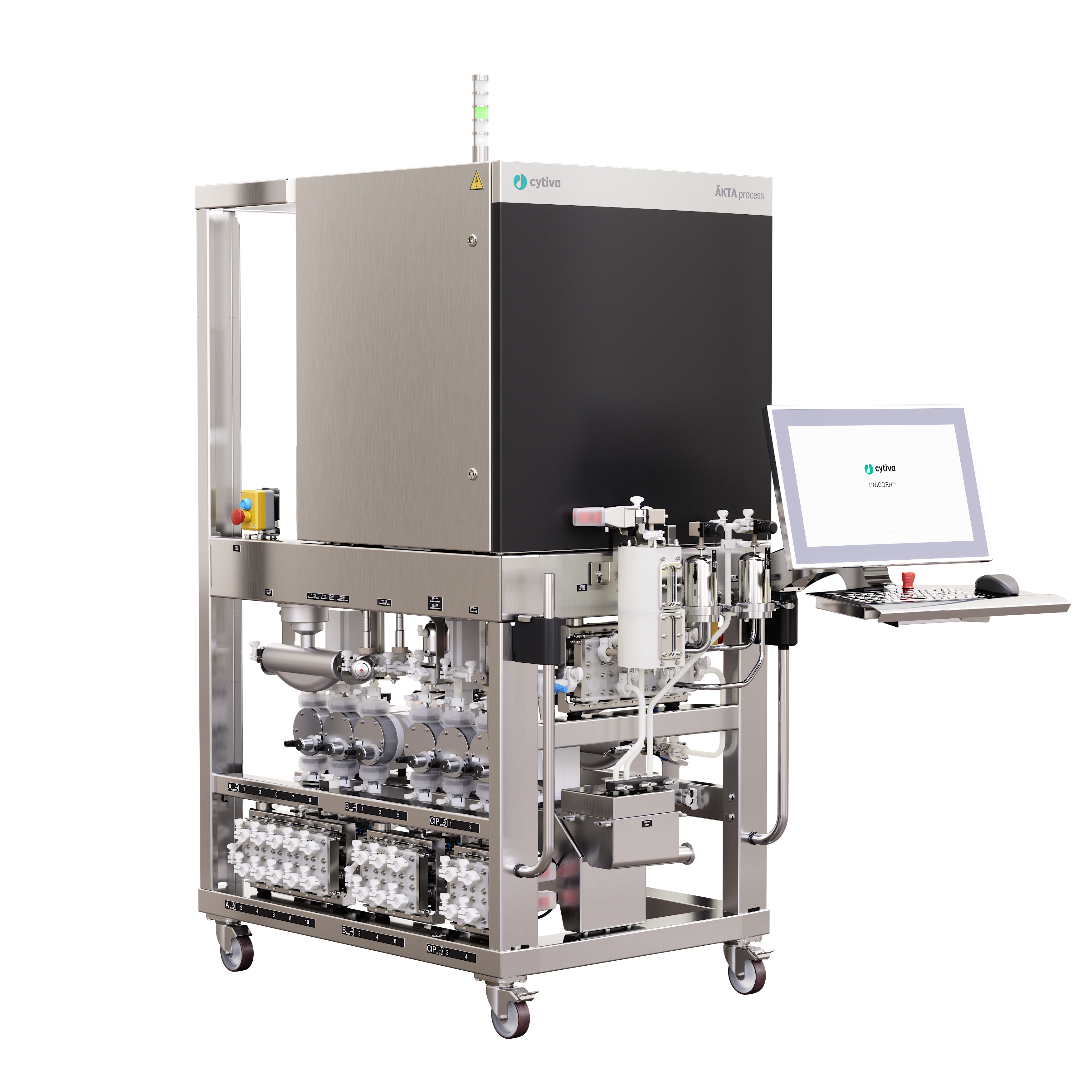
Fig 1. ÄKTA process™ chromatography system.

ÄKTA process™ is an automated large-scale chromatography system that is available in three different flow rate ranges. The flow path is available with either electropolished stainless steel or polypropylene process piping. The systems can be equipped with two high-performance membrane pumps. The pumps enable creation of accurate and reproducible binary gradients at all flow rates and pressures allowed within the system. Maximum flow rate and maximum operating pressures are shown in Table 1. ÄKTA process™ chromatography systems also have an option for a third pump that supports inline dilution (ILD).

Table 1. Maximum flow rate and maximum operating pressure of ÄKTA process™ systems

Size piping	Flow rate (L/h)	Maximum pressure (bar*)
6 mm polypropylene	1 to 180	6
10 mm polypropylene	3 to 600	6
1 in. polypropylene	10 to 2000	6
3/8 in. stainless steel	1 to 180	10
1/2 in. stainless steel	3 to 600	10
1 in. stainless steel	10 to 2000	6

*1 bar = 0.1 MPa = 14.5 psi

Designation of flow accuracy

Flow accuracy can be specified either as percentage of full scale (% FS) or as percentage of reading (% RD), or a combination of both. If an instrument has a flow accuracy specified as % FS, the error will be of a fixed value irrespective of flow rate. For example, if the full-scale flow rate is 1000 L/h and the system has an accuracy of 2% FS, the deviation will be ± 20 L/h at all flow rates.

This means that at a flow rate of 100 L/h, the deviation will also be ± 20 L/h (or ± 20% deviation from the read value). If a system instead has a flow accuracy specified as % RD, the error will always be the same percentage of the read value. In such a case, with a system accuracy of 2% RD, the deviation would be ± 20 L/h at a flow rate of 1000 L/h, but only ± 2 L/h at 100 L/h.

Designation of gradient accuracy and gradient acceptance range

Gradients are created when solutions from two or more origins are mixed into one solution at some mixing point. Gradients can be divided into two groups, linear gradients and step gradients. Gradient accuracy is often presented as a gradient acceptance range, with a defined accuracy within the acceptance range (Fig 2). The gradient acceptance range is given as % of buffer B (% B) over the flow rate range of the system.

The gradient acceptance range is based on the flow accuracy of each of the two pumps creating the gradient. One of the pumps reaches the minimum flow rate at the beginning and end of a linear gradient going from 0 to 100% B. As the flow rate goes down this narrows the acceptance range in the high and low % B area where one pump has a low flow. Outside the acceptance range the accuracy gets gradually less accurate in the high and low % B area as the flow rate is decreased. The gradient accuracy is defined as the deviation from % B within the acceptance range.

Gradient accuracy can also be shown as a chromatogram (Fig 3). The chromatogram is usually presented as the programmed % B and the actual % B at a single flow rate. The higher the flow rate, the lower the volume between mixing point and column, and the longer the gradient formation time, the better the gradient performance of the system.

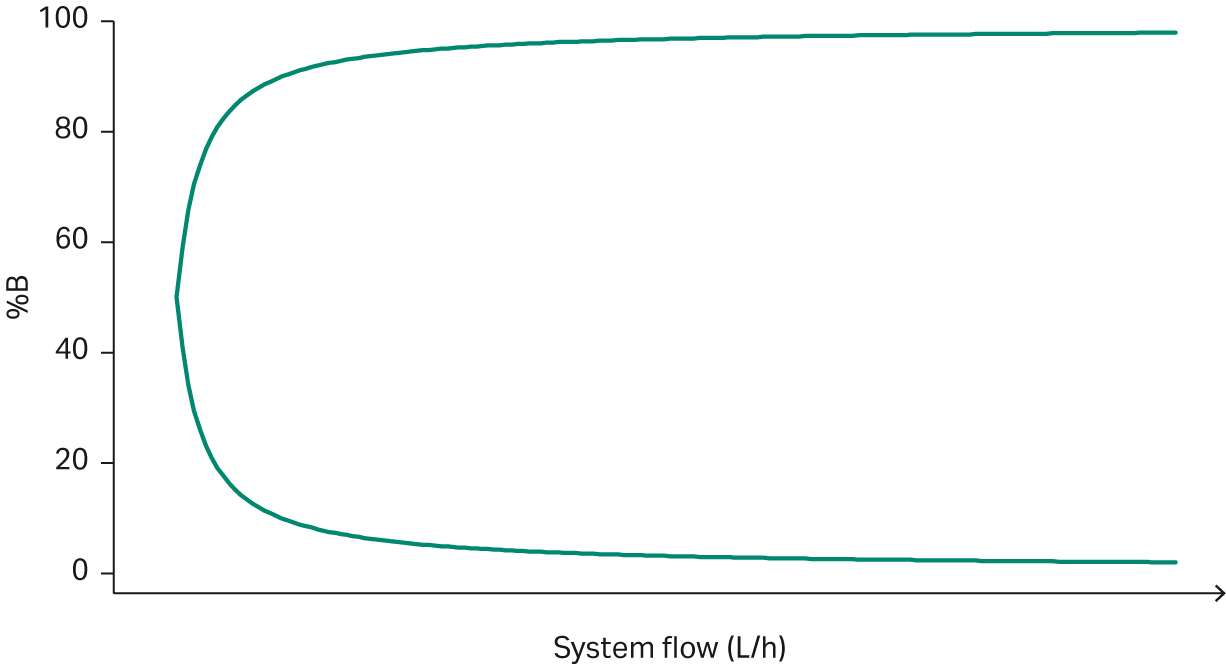
Fig 2. Example of a gradient acceptance range.

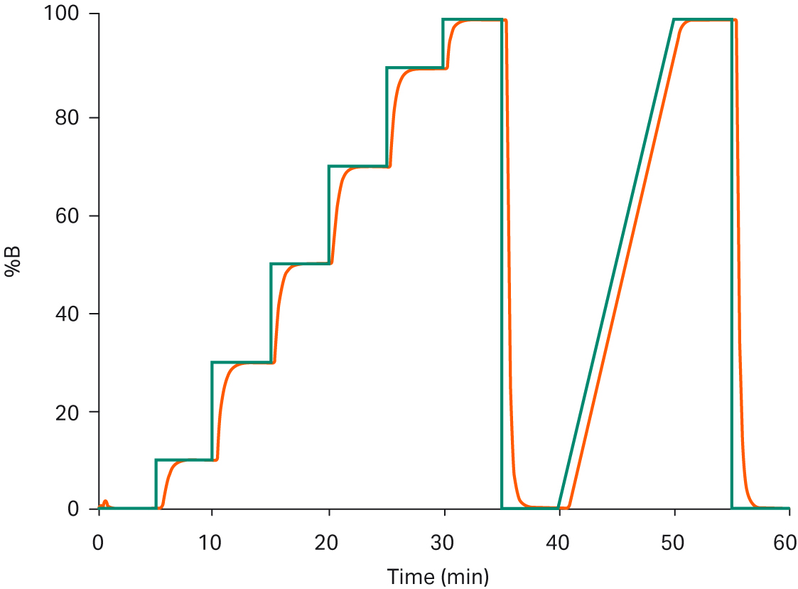
Fig 3. Example of gradient accuracy with the programmed gradient in green and the actual gradient in red.

Considerations when defining gradients

When defining a gradient, it is important to consider the gradient delay volume, that is, the volume between the mixing point and the column. The gradient delay volume is affected by all components between the mixing point and the column, such as, the air trap, filter, and the internal diameter (i.d.) of the tubing. Higher flow rates, smaller gradient delay volumes, and smaller tubing inner dimension will improve the gradient performance.

In Figure 3, the gradient is shown over time, and the delay volume can be seen as the offset of the programmed and actual gradient. A perfect gradient should follow the programmed gradient without deviation. Large hold-up volumes will create off-set between programmed and actual gradient. As can be seen in Figure 3 the actual gradient steps have a smooth curvature until the graph flattens out at the point where the gradient is fully reached. This is mostly due to the large volume of the air trap and filter. To fully exchange a buffer in an air trap, a buffer volume several times the volume of the air trap is needed.

Gradients when scaling up/down

When scaling your method up, the system volume (tubing, air trap, and filter) must be considered, especially the air trap and filter volumes. Every time a buffer change is made with the air trap and filter in-line, several times their volume is needed to fully exchange the buffer. To avoid this, the air trap and filter can be set to bypass, but this is usually not desirable and not needed at higher flow rates.

Another way to remove the differences in step gradient behavior between systems is to perform a system wash step. A system wash step is made with the column in bypass, at every buffer change where the air trap and filter need to be in-line. This will give a better effect than putting the air trap in bypass, but it requires some extra buffer. Both these ways of performing a gradient will prevent the loosely attached molecules from starting to elute before the elution-buffer has reached the target concentration. Figure 4 illustrates the difference in step gradient when the air trap is in bypass and in-line.

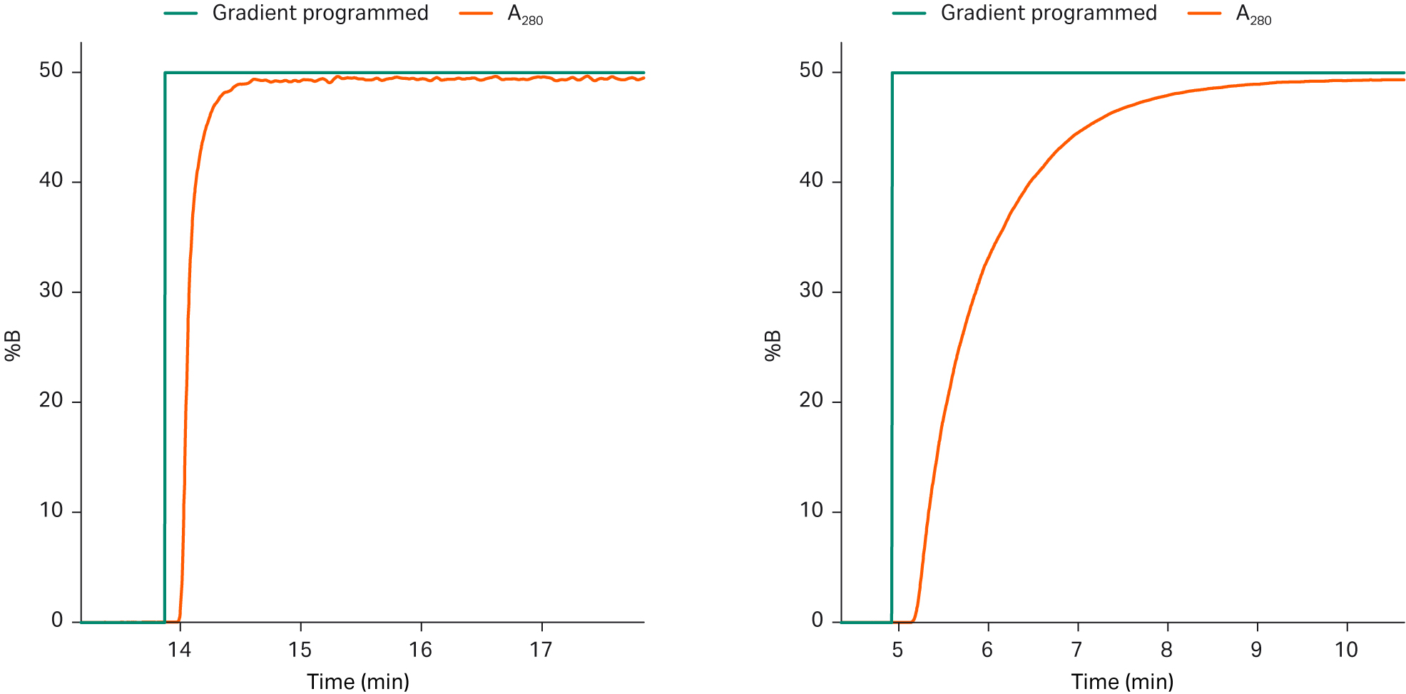
Fig 4. Comparison of a step gradient where the air trap is in bypass (left graph) and in-line (right graph) for a 6 mm system run at 90 L/h.

Results

ÄKTA process™ flow accuracy

The ÄKTA process™ 1 in. system has a flow accuracy of ±1% RD or 1 L/h, whichever is greatest. The smaller systems have a flow accuracy of ±1% RD or 0.1 L/h, whichever is greatest (Table 2).

Table 2. Flow accuracy of the ÄKTA process™ systems

Piping	Data
6 mm polypropylene	±1% RD or 0.1 L/h, whichever is greatest
10 mm polypropylene	±1% RD or 0.1 L/h, whichever is greatest
1 in. polypropylene	±1% RD or 1 L/h, whichever is greatest
3/8 in. stainless steel	±1% RD or 0.1 L/h, whichever is greatest
1/2 in. stainless steel	±1% RD or 0.1 L/h, whichever is greatest
1 in. stainless steel	±1% RD or 1 L/h, whichever is greatest

ÄKTA process™ gradient accuracy

The ÄKTA process™ system has a gradient control accuracy of ±1% B within the calculated acceptance range for the gradient if the B buffer contribution is controlled with flow. When controlling the gradient using conductivity feedback, which results in slower feedback, the accuracy is ± 2% B. This was tested by measurements at several gradient settings and on all different ÄKTA process™ systems. The measured gradient acceptance range is illustrated for the different ÄKTA process™ systems in Figures 5 through 7.

At low flow rates the full extent of a gradient (0 to 100% B) cannot be performed with accuracy since the lower and higher % B will be outside the acceptance range and hence less accurate. For this reason, we advise you to use a step gradient or narrower linear gradients within the acceptance range when low flow is used. Outside the acceptance range, the accuracy gradually decreases as the flow decrease.

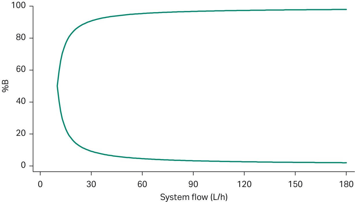
Fig 5. Measured gradient acceptance range in % B over the flow range for a standard gradient using a 6 mm system.

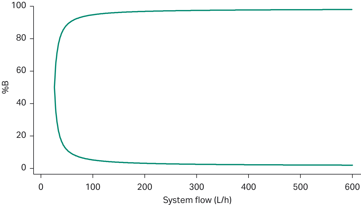
Fig 6. Measured gradient acceptance range in % B over the flow range for a standard gradient using a 10 mm system.

Fig 7. Measured gradient acceptance range in % B over the flow range for a standard gradient using a 1 in. system.

Programmed and actual gradient chromatograms with flow feedback

Figures 8 through 10 show the programmed % B and the results for the three system sizes when using flow feedback to control pump B.

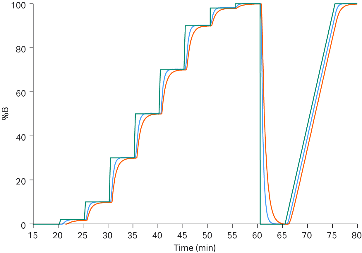
Fig 8. The chromatogram shows a 6 mm system with the programmed gradient in green, and the actual gradient at a flow rate of 180 L/h in blue and at 90 L/h in red.

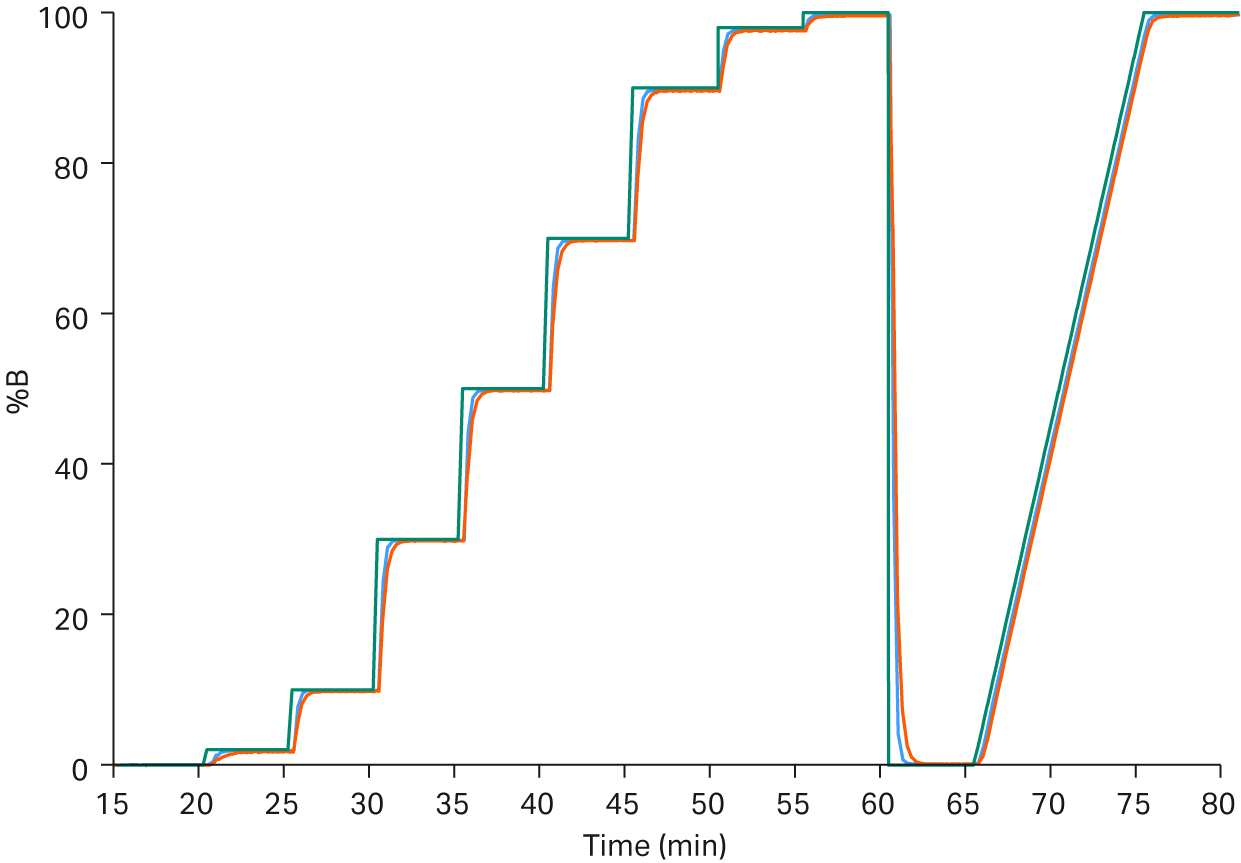
Fig 9. The chromatogram shows a 10 mm system with the programmed gradient in green, and the actual gradient at a flow rate of 600 L/h in blue, and at 300 L/h in red.

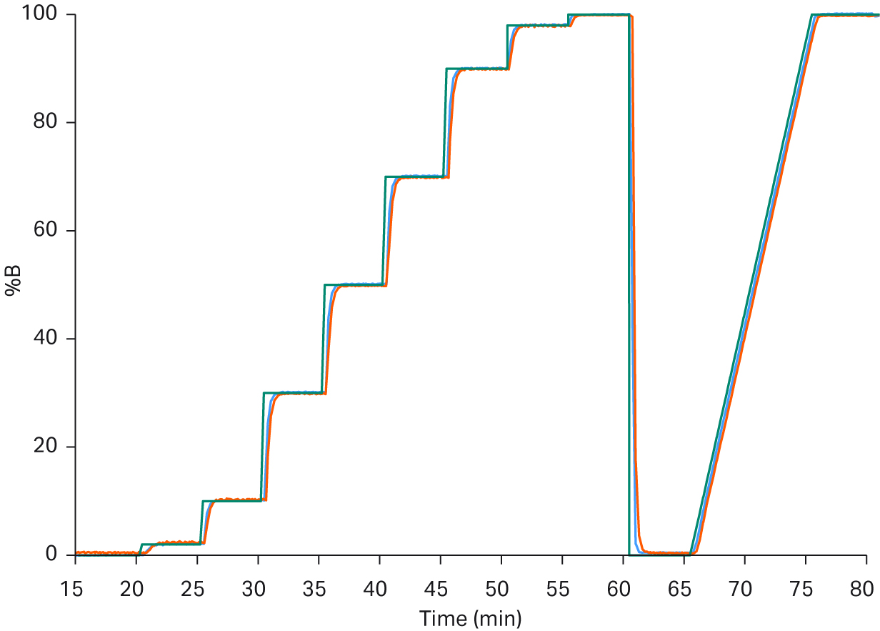
Fig 10. The chromatogram shows a 1 in. system with the programmed gradient in green, and the actual gradient at a flow rate of 2000 L/h in blue, and at 1000 L/h in red.

Programmed and actual gradient chromatograms with conductivity feedback

Figures 11 through 13 show the chromatograms for the programmed % B and results for the three system sizes when using conductivity feedback to control pump B.

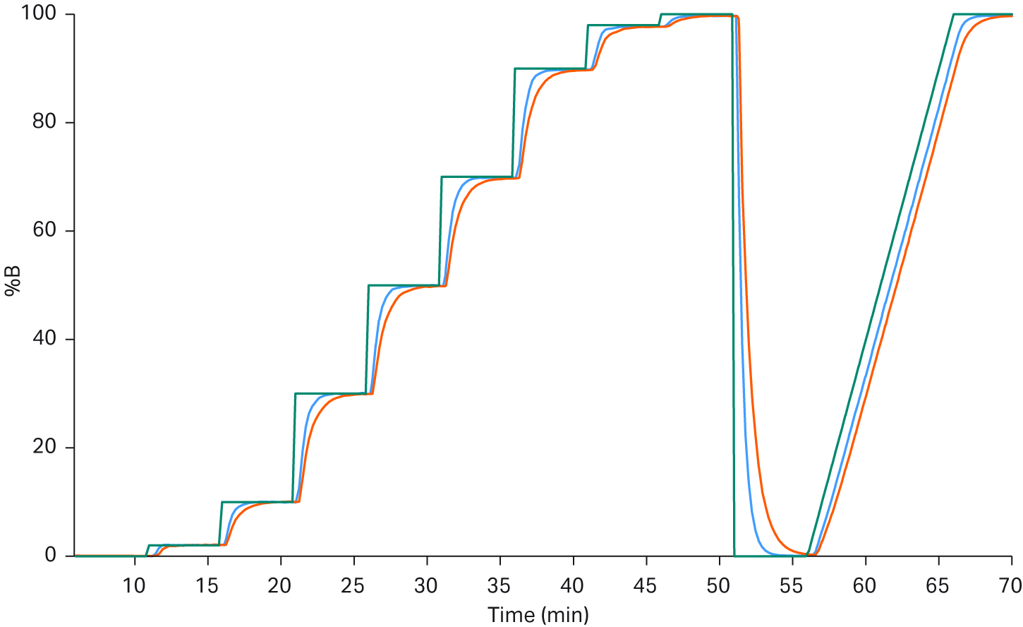
Fig 11. The chromatogram shows a 6 mm system with the programmed gradient in green, and the actual gradient at a flow rate of 180 L/h in blue and at 90 L/h in red.

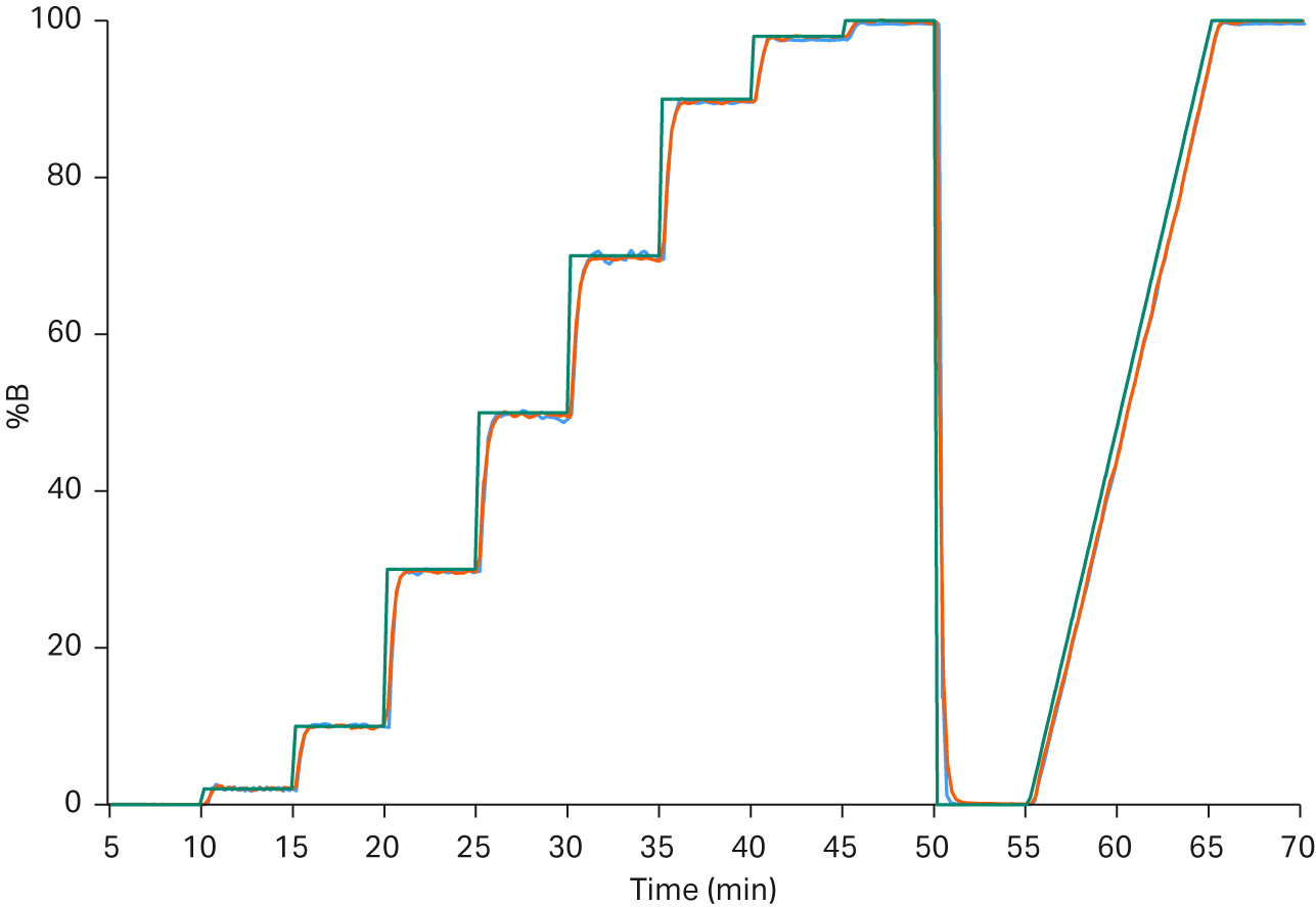
Fig 12. The chromatogram shows a 10 mm system with the programmed gradient in green, and the actual gradient at a flow rate of 600 L/h in blue and at 300 L/h in red.

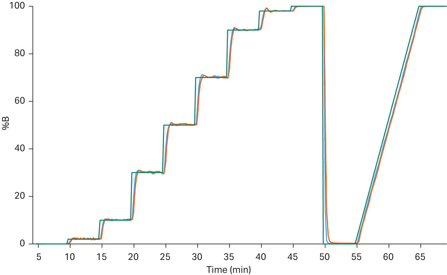
Fig 13. The chromatogram shows a 1 in. system with the programmed gradient in green, and the actual gradient at a flow rate of 2000 L/h in blue and at 1000 L/h in red.

Gradient performance

A comparison overlay of the three system sizes showing a gradient step at half the maximum flow rate for each system is shown in Figure 14. The Figure shows that it takes longer for the smaller system to start and finalize the gradient step. As previously discussed, when scaling up or down, the delay to start a gradient step is due to system volume and the delay it takes to finalize the step is due to the volume of air trap and filter.

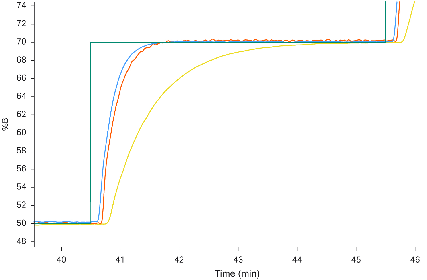
Fig 14. The graph shows a closeup of one step of the gradient with overlays of the three system sizes running at half the maximum flow rate of the respective system. The blue curve is a flow of 1000 L/h on a 1 in. system, red is 300 L/h on a 10 mm system, and green is 90 L/h on a 6 mm system.

Figure 14 also shows that a step that can be made in only 1 min on one system has to be elongated to about 5 min on another, mainly due to the effectiveness of buffer exchange in the air trap.

Conclusion

In this article, we have shown the flow and gradient accuracy of ÄKTA process™ chromatography systems.

• We have shown that the flow accuracy of ÄKTA process™ chromatography systems was found to be ± 1% RD.
• Gradient accuracy with flow feedback was found to be 1% B within the gradient acceptance range, or with conductivity feedback 2% B.
• The high accuracy over different flow rates and pressures shows that ÄKTA process™ systems have a highly stable performance.
• The high accuracy of ÄKTA process™ chromatography systems make them well-suited for scale-up and production in an GMP environment.

Learn more about ÄKTA process™ chromatography system