A typical bioprocess workflow requires many buffers and process liquids in large volumes, making buffer preparation one of the most resource-intensive activities in biomanufacturing facilities.
Here, we discuss the accuracy and performance of the inline dilution (ILD) technology found in the ÄKTA process™ chromatography system. We also compare the process economy of ILD versus manual buffer preparation — which is still the most common way to prepare buffers — by looking at the labor time, buffer volumes, floor space, and required investments for each approach.
Introduction: A summary of inline dilution and its benefits
With ILD, buffer volumes are reduced using buffer concentrates that are diluted inline with water for injection (WFI) to meet a targeted final buffer composition (Fig 1). For systems with chromatography and ILD functionality, batch sizes are smaller and buffer preparation is directly integrated into chromatography processes, eliminating the need for intermediate storage in buffer bags or holding tanks. Buffer concentrates can be prepared in-house or outsourced.
ILD can significantly reduce time, labor, and space requirements without compromising buffer quality or consistency. To be successful, ILD requires accurate sensors and pumps with wide flow ranges.
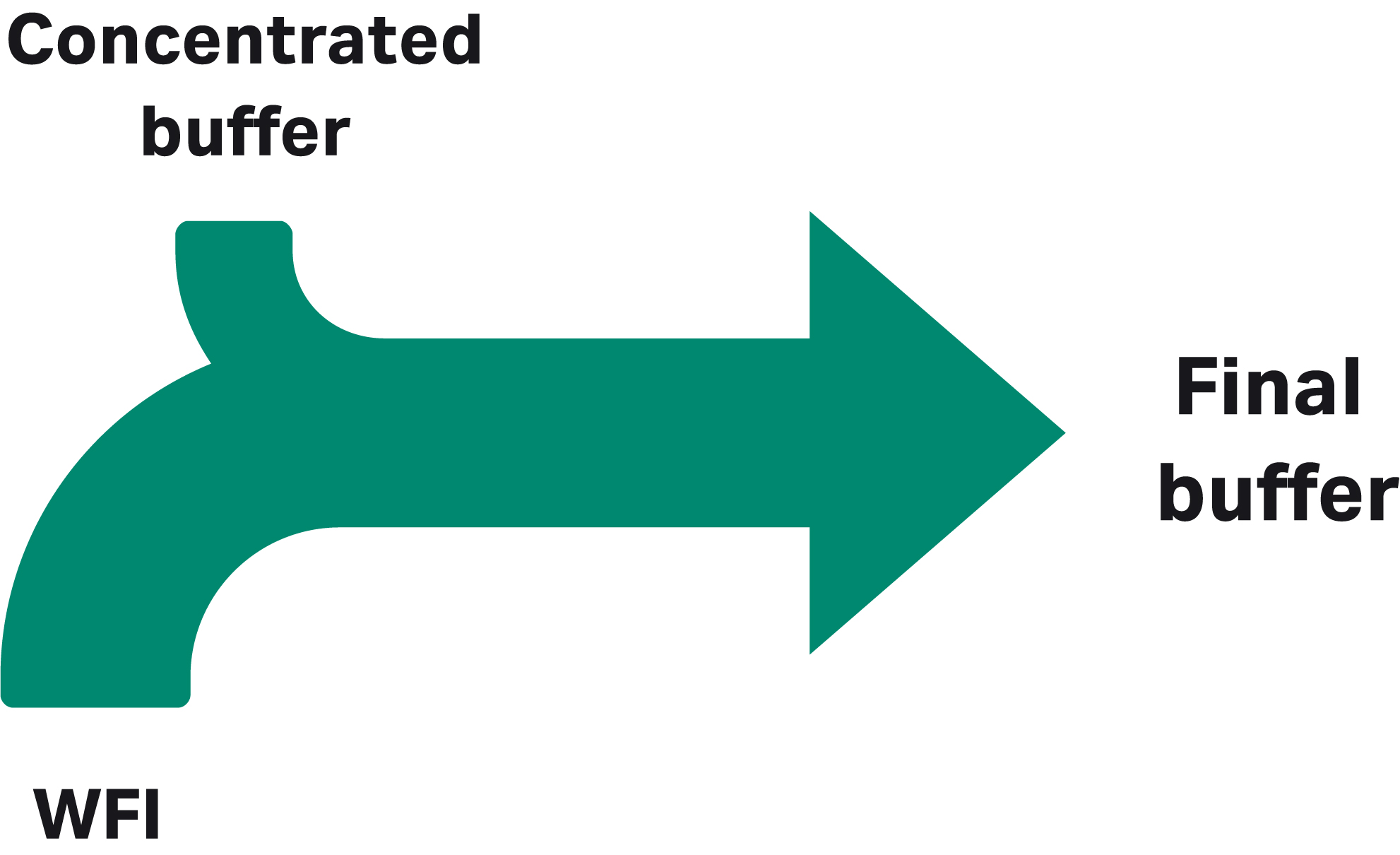
Fig 1. With ILD, buffer volumes can be reduced by using buffer concentrates diluted inline with water for injection.
ÄKTA process™ chromatography system with inline dilution
The automated ÄKTA process™ liquid chromatography system is built for process scale-up and large-scale biopharmaceutical manufacturing. It is available in three different flowrate ranges from 1 L/h to 2000 L/h with a flow path made of either electropolished stainless steel or polypropylene (Table 1). This system provides the accuracy and documentation needed for GMP-regulated environments, and serves as a good choice for scaling up and transferring processes developed on smaller ÄKTA™ chromatography systems.
The ÄKTA process™ chromatography system offers a flexible design that can be easily configured to meet different process demands, including the option of adding a third pump to support ILD for buffer preparation (Fig 2). By combining the ÄKTA process™ chromatography system with ILD, buffers can be prepared and sourced at the point of use, leading to space, time, and cost savings.
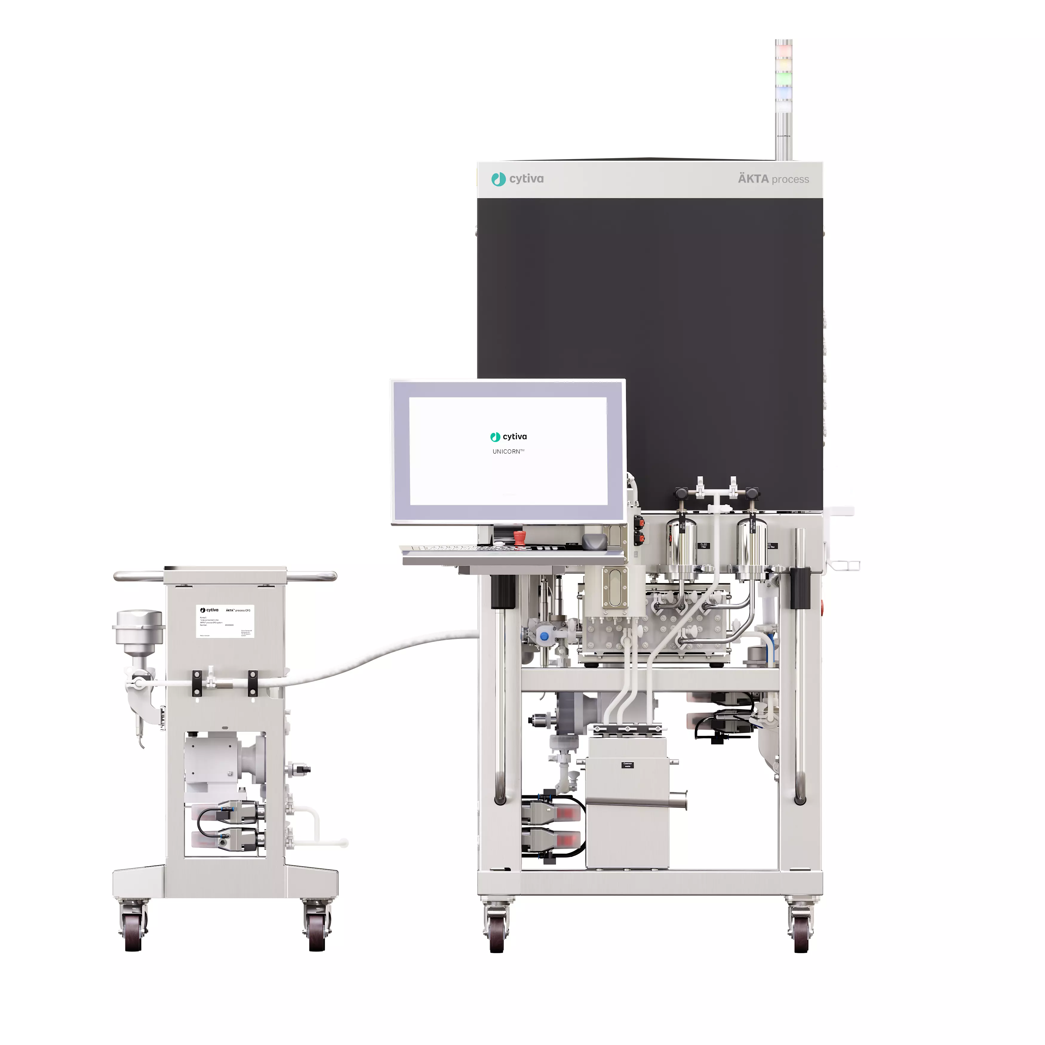
Fig 2. ÄKTA process™ chromatography system with the third pump that supports inline dilution (ILD).
Table 1. Maximum flow rate and maximum operating pressure of ÄKTA process™ systems
| Piping size and material | Flow rate (L/h) | Maximum pressure (bar) |
|---|---|---|
| 6 mm polypropylene | 1 – 180 | 6 |
| 10 mm polypropylene | 3 – 600 | 6 |
| 1 inch polypropylene | 10 – 2000 | 6 |
| 3/8 inch stainless steel | 1 – 180 | 10 |
| 1/2 inch stainless steel | 3 – 600 | 10 |
| 1 inch stainless steel | 10 – 2000 | 6 |
1 bar = 0.1 MPa = 14.5 psi
Using ÄKTA process™ system for inline dilution
To perform ILD with an ÄKTA process™ chromatography system, the third pump dilutes the buffer concentrates coming from the A and B pumps. A user can set a dilution factor for the third pump, ranging between 1 and 100 times. The third pump will then dilute the buffers coming from the A and B pumps to the set dilution factor. This process can also be managed by other control systems, like the DeltaV™ Distributed Control System (DCS).
The accuracy of the gradient is dependent on the accuracy of the signal used for gradient feedback control. The actual gradient in ILD is therefore dependent on the flow meter’s accuracy. The concentrated buffers should also be formulated precisely.
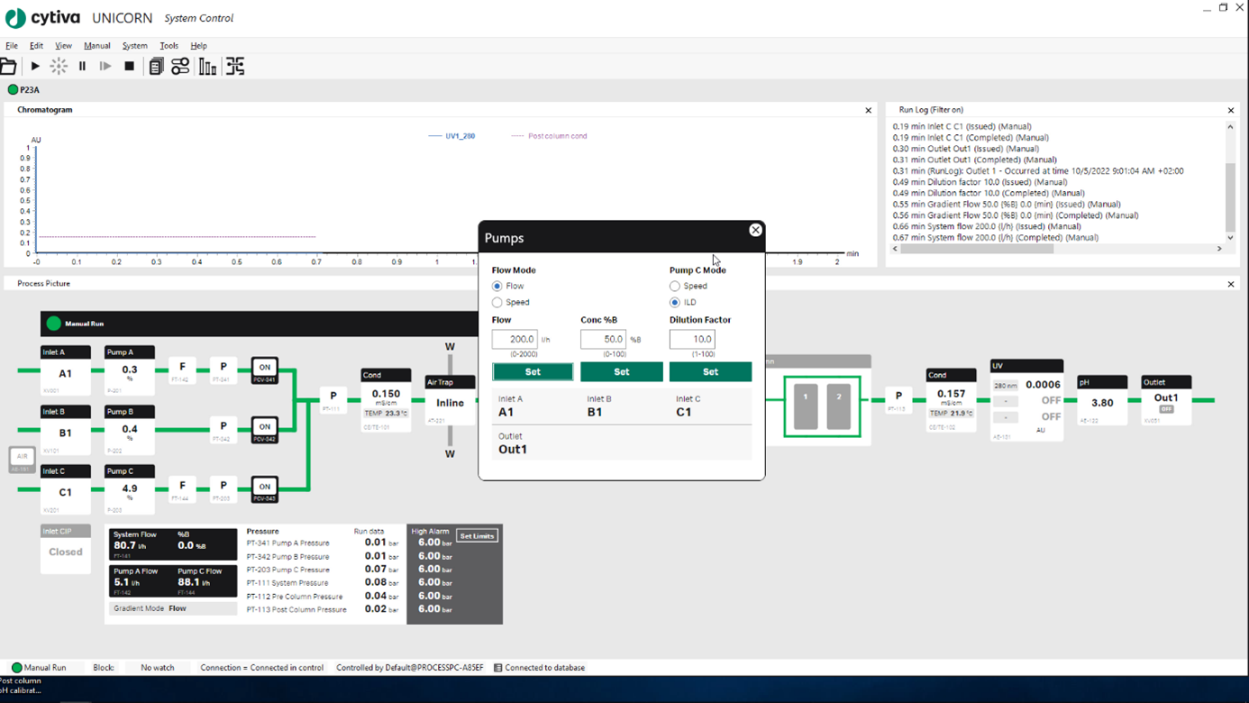
Fig 3. The ÄKTA process™ chromatography system with UNICORN™ software provides an interactive process picture. The ILD functionality can also be viewed and controlled through this software.
Accuracy and performance
Designation of flow accuracy
Flow accuracy can be specified either as percentage of full scale (% FS) or as percentage of reading (% RD), or a combination of both. If an instrument has a flow accuracy specified as % FS, the error will be of a fixed value irrespective of flow rate. For example, if the full-scale flow rate is 1000 L/h and the system has an accuracy of 2% FS, the deviation will be ± 20 L/h at all flow rates. This means that at a flow rate of 100 L/h, the deviation will also be ± 20 L/h (or ± 20% deviation from the read value).
If a system instead has a flow accuracy specified as % RD, the error will always be the same percentage of the read value. In such a case, with a system accuracy of 2% RD, the deviation would be ± 20 L/h at a flow rate of 1000 L/h, but only ± 2 L/h at 100 L/h.
Designation of gradient accuracy and gradient acceptance range
Gradients are created when solutions from two or more origins are combined into one solution at some mixing point. Gradients can be divided into two groups: linear gradients and step gradients. Gradient accuracy is often presented as a gradient acceptance range, with a defined accuracy within the acceptance range. The gradient acceptance range is given as % of buffer B (% B) over the flow rate range of the system.
The gradient acceptance range is based on the flow accuracy of each of the pumps creating the gradient. One of the pumps reaches the minimum flow rate at the beginning and end of a linear gradient, going from 0% to 100% B. As the flow rate goes down, the acceptance range narrows down in the high and low % B area where one pump has a low flow. Outside of the acceptance range, the accuracy gradually decreases in the high and low % B area as the flow rate is decreased. The gradient accuracy is defined as the deviation from % B within the acceptance range.
Results
Flow accuracy of the ÄKTA process™ system with ILD
When using flow feedback, the ÄKTA process™ 1-inch system with ILD has a flow accuracy of ±1% RD or 1 L/h, whichever is greatest, and the smaller systems have a flow accuracy of ±1% RD or 0.1 L/h, whichever is greatest. (Table 2)
Table 2. Flow accuracy of the ÄKTA process™ systems
| Piping size and material | Flow accuracy |
|---|---|
| 6 mm polypropylene | ±1% RD or 0.1 L/h, whichever is greatest |
| 10 mm polypropylene | ±1% RD or 0.1 L/h, whichever is greatest |
| 1 inch polypropylene | ±1% RD or 1, L/h whichever is greatest |
| 3/8 inch stainless steel | ±1% RD or 0.1, L/h, whichever is greatest |
| 1/2 inch stainless steel | ±1% RD or 0.1, L/h whichever is greatest |
| 1 inch stainless steel | ±1% RD or 1, L/h whichever is greatest |
Gradient accuracy of ÄKTA process™ system with ILD
The ÄKTA process™ system with ILD has a gradient-controlled accuracy of ±2% B within the gradient acceptance range. We tested this by taking measurements at three different dilution factors and three different flowrates on all three system sizes. The gradient acceptance ranges at the points of measurement are illustrated for the three system sizes in Figures 4 through 6.
When referring to control accuracy, we mean the deviation between the theoretical gradient and the signal used for feedback control of the gradient. In flow mode, this is the flow rate measured by the flow meters; for conductivity-controlled mode, this is the conductivity read by the pre-column conductivity monitor. The actual gradient is thus dependent on how accurately the conductivity monitor, for example, is calibrated.
At a low flow rate or high dilution factor, the full extent of a gradient (0% to100% B) will, at the beginning and end, be outside of the acceptance range where accuracy is not as good. Outside of the acceptance range, the accuracy gradually decreases in the high and low % B area or with a higher dilution factor, as the flow rate is decreased, and it is advised to use a step gradient or narrower linear gradients within the acceptance range.
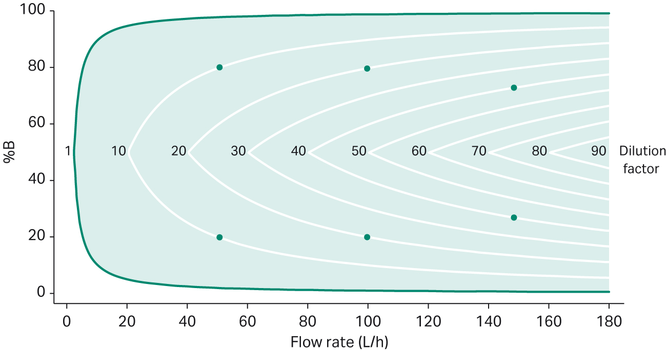
Fig 4. Gradient acceptance range in % B over the flow range for a 6 mm ÄKTA process™ system with ILD at different dilution factors (10, 20, 30, 40, 50, 60, 70, 80). The gradient-controlled accuracy within the acceptance ranges is ±2% B. The dots on the curves with dilution factors 10, 20, and 40 indicate the measured minimum and maximum gradient compositions at specific flow rates, also described in Table 3.
Table 3. Measured gradient compositions at given flow rates and dilution factors for a 6 mm ÄKTA process™ system with ILD (marked as dots in the Figure 4)
| Flow rate (L/h) | Dilution factor | Gradient min/max composition (%) |
|---|---|---|
| 50 | 10 | 20 – 80 |
| 100 | 20 | 20 – 80 |
| 150 | 40 | 27 – 73 |
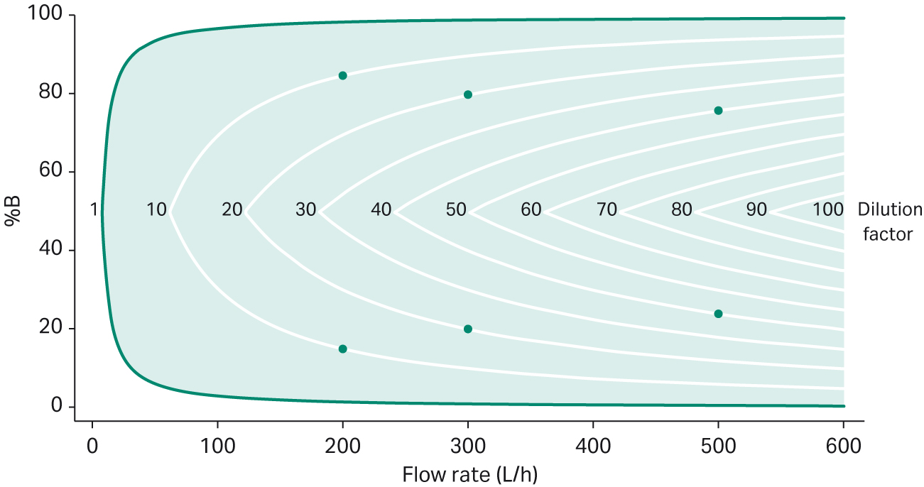
Fig 5. Gradient acceptance range in % B over the flow range for a 10 mm ÄKTA process™ system with ILD at different dilution factors (10, 20, 30, 40, 50, 60, 70, 80, 90). The gradient-controlled accuracy within the acceptance ranges is ±2% B. The dots on the curves with dilution factors 10, 20, and 40 indicates the measured minimum and maximum gradient compositions at specific flow rates, also described in Table 4.
Table 4. Measured gradient compositions at given flow rates and dilution factors for a 10 mm ÄKTA process™ system with ILD (marked as dots in Figure 5)
| Flow rate (L/h) | Dilution factor | Gradient min/max composition (%) |
|---|---|---|
| 200 | 10 | 15 – 85 |
| 300 | 20 | 20 – 80 |
| 500 | 40 | 24 – 76 |
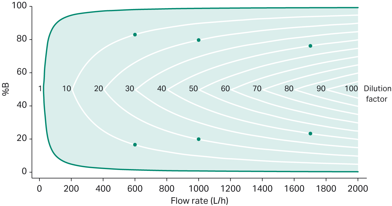
Fig 6. Gradient acceptance range in % B over the flow range for a 1-inch ÄKTA process™ system with ILD at different dilution factors (10, 20, 30, 40, 50, 60, 70, 80, 90). The gradient-controlled accuracy within the acceptance ranges is ±2% B. The dots on the curves with dilution factors 10, 20, and 40 indicate the measured minimum and maximum gradient compositions at specific flow rates, also described in Table 5.
Table 5. Measured gradient compositions at given flow rates and dilution factors for a 1-inch ÄKTA process™ system with ILD (marked as dots in Figure 6)
| Flow rate (L/h) | Dilution factor | Gradient min/max composition (%) |
|---|---|---|
| 600 | 10 | 17 – 83 |
| 1000 | 20 | 20 – 80 |
| 1700 | 40 | 24 – 76 |
Process economy comparisons between ILD and manual buffer preparation
Here, we take a closer look at how the process economy differs when buffers are prepared manually versus with ILD using in-house or outsourced buffer concentrates, like HyClone™ buffer concentrates (Fig 7). We compare labor time, volumes handled, minimum required floor space, and required capital investments for these three buffer preparation strategies.
Calculations are based on a typical three-step monoclonal antibody (mAb) process with 40 batches per year, requiring 15 000 L of buffers per batch.
All process economy calculations are indicative and based on data from 2021. The calculations are derived from Cytiva’s internal total cost of ownership tool.
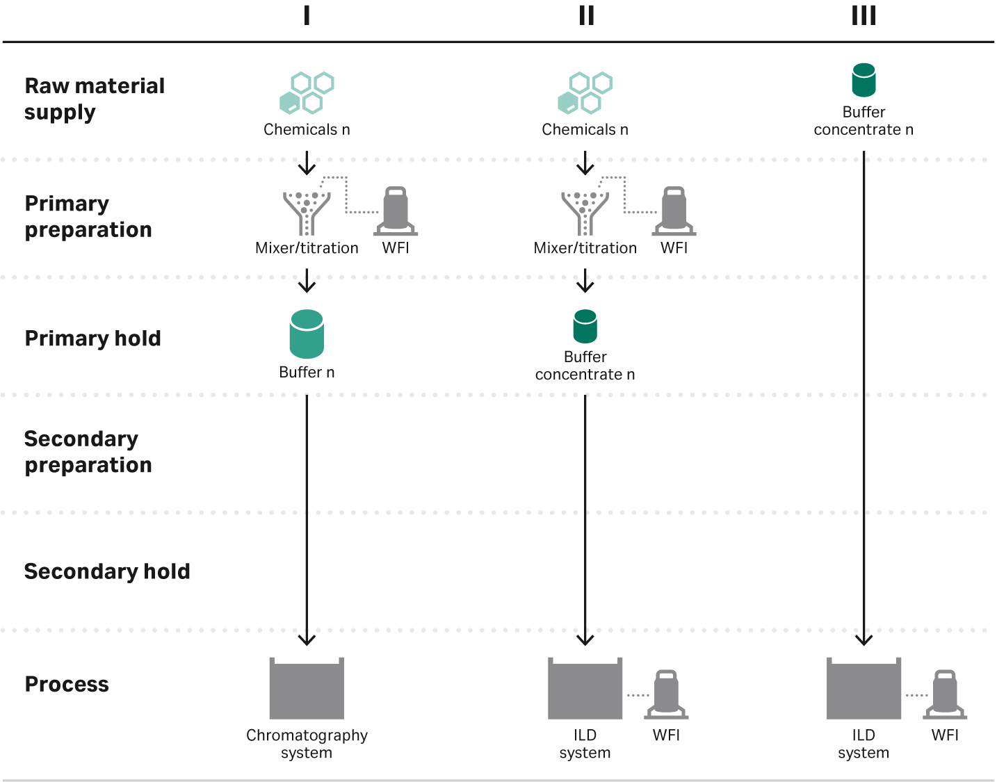
Fig 7. Buffer preparation workflows for manually prepared buffers (I), buffers prepared with ILD using buffer concentrates that have been prepared in-house (II), and buffers prepared with ILD using outsourced buffer concentrates (III).
Process economy calculations
When considering the time and labor needed to prepare buffers per batch, the difference between manual preparation versus ILD is significant, especially when ILD is coupled with outsourced buffer concentrates. Manual buffer preparation requires nearly 400 hours for one buffer batch of 15 000 L, ILD with in-house prepared buffer concentrates requires over 300 hours, and ILD with outsourced buffers under 20 hours.
When comparing cumulative costs — including capital investment, operational costs, and depreciation over 10 years — our calculated estimates suggest that ILD with manually prepared buffers is around 15% and ILD with outsourced buffer concentrates is around 40% more cost-efficient than manual buffer preparation after ten years. In fact, the economic benefits of ILD become clear after just the first year. The use of buffer concentrates with ILD is the most economical option long-term of the methods we compared, as the primary preparation and primary hold steps can be skipped completely.
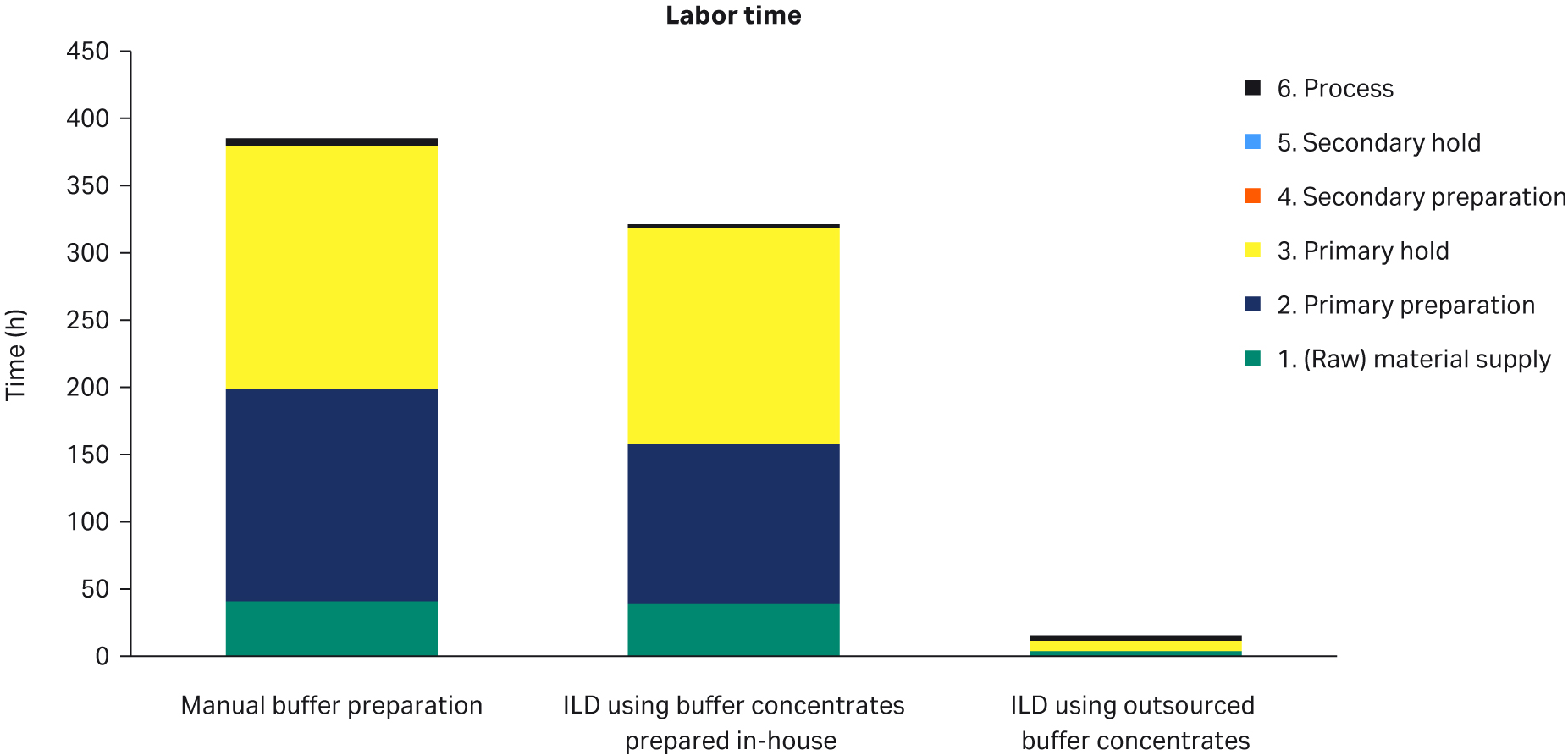
Fig 8. Buffer preparation workflows for manually prepared buffers (I), buffers prepared with ILD using buffer concentrates that have been prepared in-house (II), and buffers prepared with ILD using outsourced buffer concentrates (III).
Also, while the total volume of buffer used per batch will be the same regardless of preparation method, the buffer volumes that need to be handled and moved outside of the chromatography system differ significantly between manual buffer preparation and ILD. With manual buffer preparation, over 33 000 L of buffer need to be managed. ILD significantly decreases this volume, as only the concentrates need to be managed and moved. With in-house prepared concentrates and ILD, the volume that needs to be handled is around 7200 L. With outsourced buffer concentrates and ILD, it is only around 3500 L.
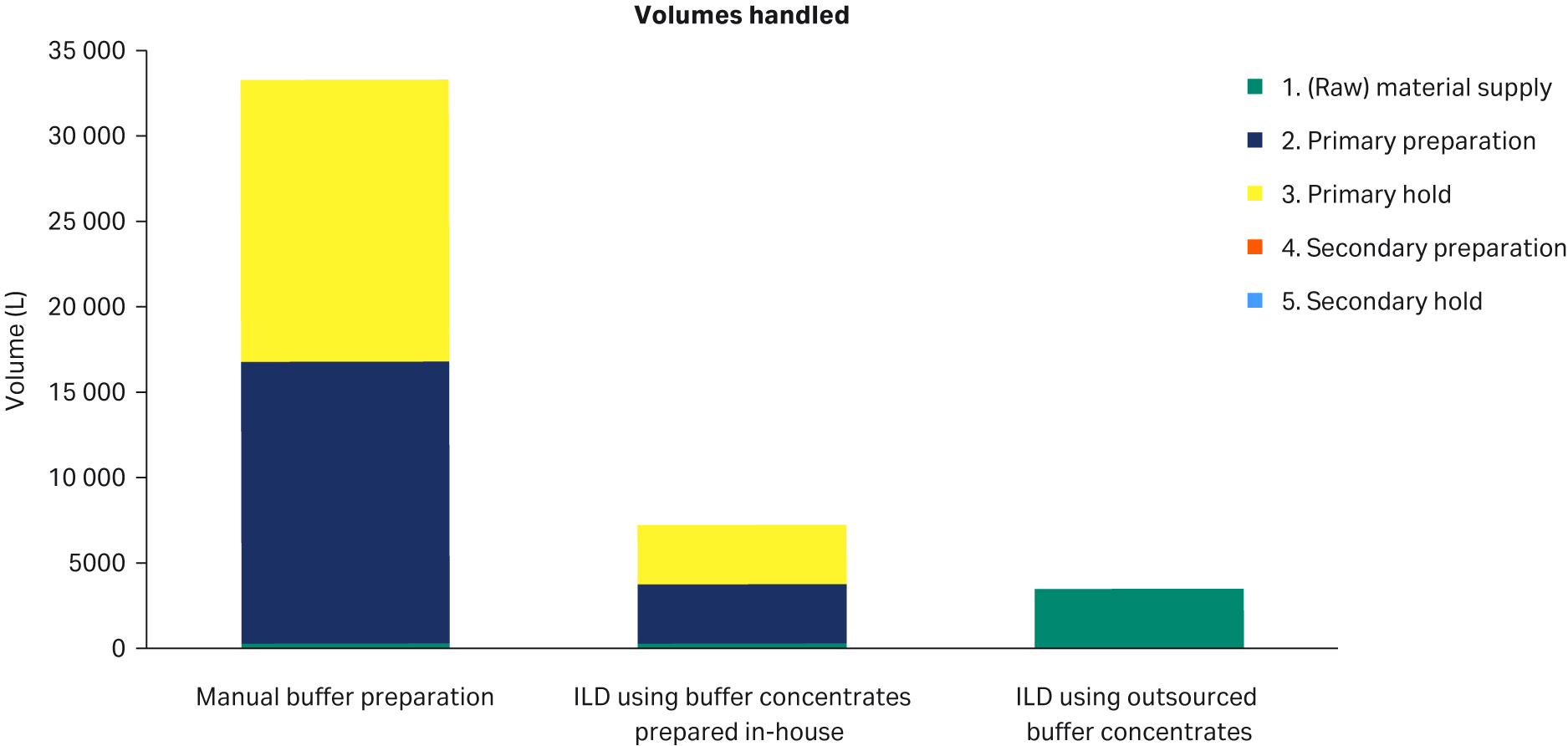
Fig 9. Buffer volumes handled per batch for each buffer preparation method.
There are also major differences in the required floor space reserved for buffer preparation when comparing these three approaches. Due to the large buffer volumes managed outside of the chromatography system, manual buffer preparation requires around 120 m2, with nearly 52 m2 required in the processing suite and 57 m2 needed in the buffer kitchen. ILD with in-house prepared buffer concentrates requires around 55 m2, and ILD with outsourced concentrates needs only around 20 m2.
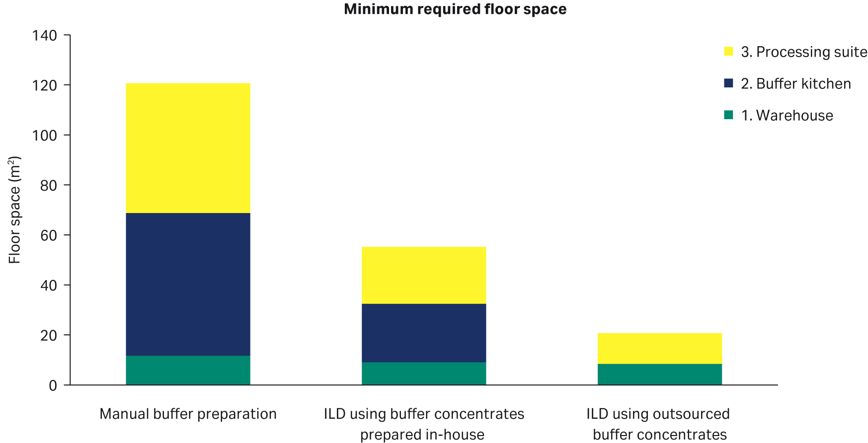
Fig 10. Minimum required floor space for each buffer preparation method.
Conclusion
Buffer management is a time-consuming activity and manual preparation of buffers can become a major bottleneck, especially when manufacturing scales increase. By implementing ILD, buffer production remains an in-house activity, but labor and space required for buffer preparation and handling are reduced by automating the preparation process and using HyClone™ buffer concentrates for additional time and space savings.
The process economy calculations in this article indicate that ILD can lead to savings in terms of investments, labor time, buffer volumes handled, and floor space requirements when compared to manual buffer preparation. The benefits of ILD become even more substantial when using outsourced buffer concentrates.
Materials and methods
We investigated the flow accuracy of the ÄKTA process™ chromatography system with ILD at different flow rates, always with 3 bar backpressures and default PID parameters. The gradient accuracy and acceptance range for different dilution factors were calculated from the flow accuracy and subsequentially tested at three dilution factors and three flow rates.