With advancing digitalization, mechanistic modeling has established itself as the method of choice for creating improved process understanding, intensified process development, and unparalleled process performance. Mechanistic models have become a very valuable technique to describe chromatography separation processes. Digital twins based on mechanistic models enable in-depth understanding of even very complex separation processes and are applicable at any point of a therapeutic product’s life cycle, reducing the cost and time for downstream process development.
However, the main hurdle within every mechanistic modeling project is the often-cumbersome approach to model calibration. Multicomponent feed stocks lead to multidimensional parameter estimation problems with many unknown biomolecule-specific thermodynamic parameters. Unsupervised model calibration approaches may result in unreasonable correlations and unrealistic physical parameter estimates.
This article outlines considerations within a standardized workflow to ensure good modeling practice. General considerations are complemented by an application example showcasing the optimization of an ion-exchange polishing step. The target biomolecule, a monoclonal antibody, was separated from charge variants using a precharacterized f(x) column for rapid calibration.
1. Set the scope

To follow good modeling practice, the first and important step is to set the scope and context of use and to define the project goal. These considerations are very important for the experimental design of the calibration runs and for the definition of a model validation strategy. It is crucial to know about the process challenges and define the expected model capability to ensure that the model will meet the desired requirements later.
Find a general guide to setting the scope here.
Case study
The scope of the study was to optimize an ion-exchange chromatography polishing. The feed is composed of ~ 72% monoclonal antibody as main species, ~ 18% acidic charge variants, and ~ 10% basic charge variant. The acceptance criteria for the process are a final pooled product with a purity of > 95%, while maintaining a yield of at least 80%. Here, the acidic variants are considered a critical impurity, while the basic variant was not classified as a critical impurity and therefore acceptable in the pooled fraction. To meet the purification requirements, a two-step method is to be optimized for process pH and for salt concentration during elution. A small elution volume and high load density are the secondary requirements for high process productivity, which are to be targeted by optimizing the load density and elution volume.2. Select variable and non-variable process parameters and chromatography setup

After defining the project scope, the variable and non-variable process parameters of the project are selected. Variable parameters are the parameters that are varied to fulfill the scope of the project (e.g., salt concentration for elution, pH at different steps of the process, or load density). The non-variable parameters refer to the chromatography setup and include, for instance, the scale of column and system used for calibration. Other non-variable parameters that are part of the chromatographic separation problem at hand may include resin type, buffer system, or suitable analytical methods to distinguish target and impurities.
Identifying the process parameters that will not be varied to achieve the defined goal of the modeling project is the first step to narrowing down the boundaries for your calibration experiments. Hereby, the setup and process parameters can be selected based on experimental knowledge and experience, for example, based on processes with a comparable molecule or a resin screening.
Case study
The chromatography setup and non-variable process parameters were selected based on prior knowledge with a comparable molecule and experimental experience.
Chromatography setup:
- System: ÄKTA pure™ 25
- Column format: Tricorn™ 10/100 f(x) column, a prepacked and precharacterized column that replaces column characterization experiments.
Non- variable process parameters:
- Process mode: bind and elute
- Resin: Capto™ SP ImpRes, a strong cation exchanger that was chosen due to its high resolution for separation of closely related charge variants that have only small differences between the target variant and the acidic species
- Resin properties: one resin lot was used
- Load composition: analyzed feed material from one batch was used
- Analytics: an existing HPLC (high performance liquid chromatography) ion exchange method was applied for analysis of target molecule and charge variants
- Buffer system: 25 mM sodium phosphate with NaCl for elution
- Flowrate: flowrate was set to 150 cm/h, corresponding to 2 mL/min.
Variable process parameters:
- Process pH: pH during binding, wash, and elution; not varied between steps
- Method: elution volume of first and second elution step
- Method: salt concentration during elution, %B for first step
- Load density: applied amount of biomolecule feed material per volume of resin
Generally, all parameters that are defined here as non-variable process parameters or are part of the chromatography setup could be defined as variable process parameters to fulfill a desired project goal. For example, varying load composition could be modeled to assess the robustness of the process. Or flowrate, system, and column dimension could be adapted to predict a process at larger scale.
3. Define boundaries for variable process parameters

The third step is identifying the boundaries for the variable process parameters that are relevant to meeting the project goal. By setting these boundaries for process parameters like pH, phase duration, or load density, we effectively narrow down the parameter space that is going to be explored to find optimal conditions. Setting these boundaries also serves as a requirement to define the experimental design for model calibration. It allows us to focus our efforts on exploring the most promising regions of the parameter space. In many cases, these boundaries can be set based on experience or existing experimental knowledge such as plate screening studies or dynamic binding capacity runs.
Case study
The following variable parameters were considered for optimization of the process:
Process pH and salt concentration during elution:
No prior knowledge on a suitable process pH range was available. The pI of the protein was known to be around pH 9. To derive a suitable pH center point and boundaries for optimization, three salt gradient elution experiments were performed in which the salt concentration was increased from 0 to 1000 mM NaCl at pH 6, pH 7 and pH 8.
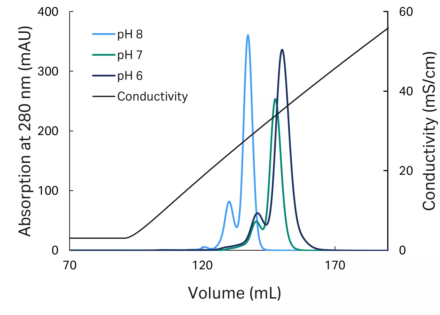
Fig 1. Process pH screening with linear gradient elution.
Observations:
- Comparable peak resolution for pH 6 and pH 7.
- Load material analysis showed increased formation of critical acidic variants at pH 8.
- Complete elution achieved below 600 mM NaCl for all tested pH values.
Conclusion:
- pH 7 was selected as center point for optimization, with boundaries of ± 0.5 pH units
- Salt concentration of buffer B (elution buffer) was set to 600 mM NaCl
Load density:
No prior knowledge on the dynamic binding capacity (DBC) of the molecule on the selected resin and pH range was available. A DBC run at the defined center point pH 7 was performed.
Observations:
- DBC at 10% breakthrough at ~ 123 g/L
Conclusion:
- Target for chromatography process optimization of at least 50% of DBC at 10% breakthrough, which equals a loading of at least 60 g/L
Based on the conclusions drawn from these prescreening experiments, the boundaries of the variable process parameters were defined, narrowing down the parameter space for optimization and providing the required input for experimental planning in the next step.
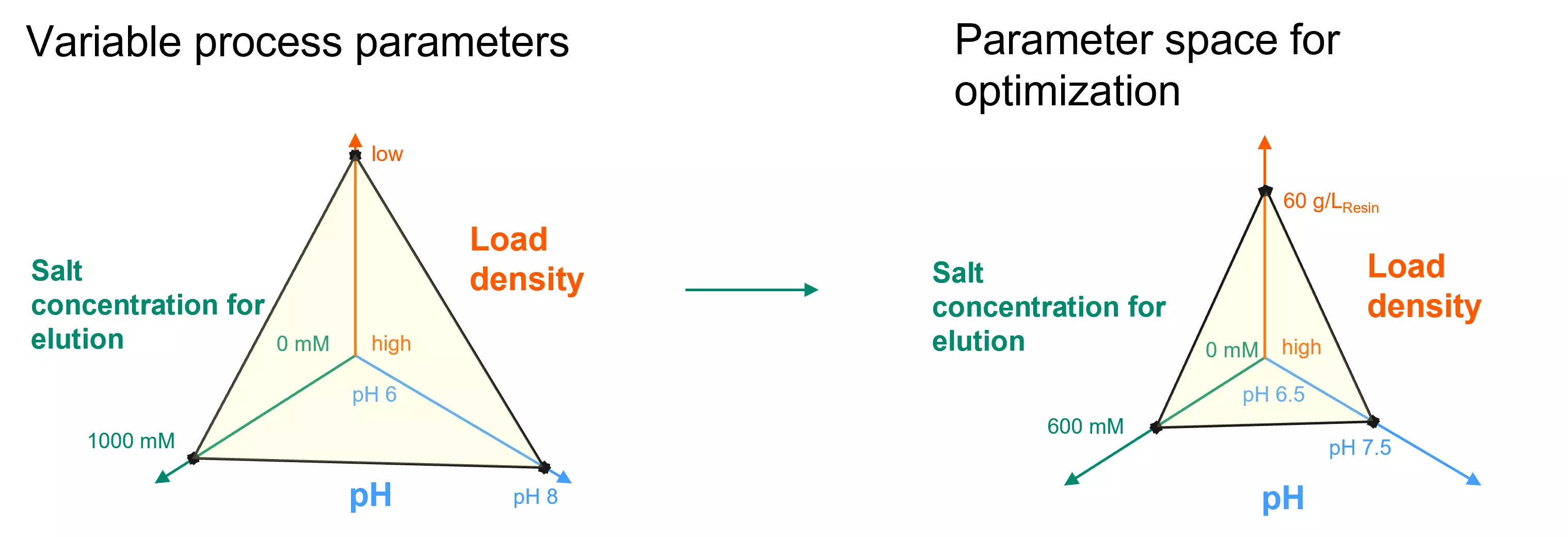
Fig 2. Parameter space before and after definition of boundaries for variable process parameters.
4. Plan and execute your calibration experiments

Experimental design and considerate execution are key to successful process development. The previously defined boundaries, project goal, and available resources should be considered for the experimental design. The aim of experiments performed for model calibration is to capture all relevant chromatographic effects and phenomena. Consequently, experimental variation (e.g., gradients and steps, high and low load density) needs to be reflected by the experimental plan.
Furthermore, the predictive power of the model relies on the experimental data it is built on. A mechanistic model for chromatography combines fluid-dynamic effects occurring in the system and column with thermodynamic effects taking place between biomolecule and ligand. To be able to describe both effects, system and column characterization experiments as well as adsorption experiments with biomolecule feed should be performed. Reliable experimental data is crucial to ensure that the calibrated model fits its purpose.
Case study
Characterization of fluid dynamics:
Fluid-dynamic effects in the system and column are captured by performing a system and column characterization. A procedure with detailed experimental outline and interpretation of results can be accessed here.
First, the system is characterized by performing a simple tracer experiment:
Table 1. System characterization
| Experiment | Parameter name | Experimental result |
| Tracer experiment with 0.8 M NaCl, 1% acetone as tracer substance, and 0.4 M NaCl in the background | System dead volume | 0.19 mL from injection valve to UV sensor 0.28 mL from injection valve to conductivity sensor |
To reduce experimental efforts for column characterization, a precharacterized Capto SP ImpRes f(x) column in Tricorn 10/100 format was selected. The f(x) columns are characterized using standardized, reliable, and consistent methods. They provide all parameters relevant for model building on the results of analysis (RofA) sheet and reduce the introduction of unwanted parameter variation for model calibration.
Table 2. Overview of required system and column parameters and experimental derivation. All parameters are provided on the RofA sheet delivered with every f(x) column.
| Parameter name | Experimental result | Unit | |
| Column geometry | Bed height | 103 | mm |
| Inner column diameter | 10 | mm | |
| Porosities | Interstitial porosity | 32 | % |
| Bead porosity | 75 | % | |
| Total porosity | 83 | % | |
| Dispersion | Axial dispersion | 0.126 | mm²/s |
Biomolecule experiments:
The following experimental plan was executed. The load density, pH, and salt concentration for step and gradient elution were set based on the previously defined boundaries. We recommend performing all calibration experiments on the same system and column to keep variations (e.g., column porosity or system flow path between calibration experiments) to a minimum.
Find general experimental guidance here.
Typically, three linear gradient elution (LGE) runs at low load density (#1 to #3), one LGE at moderate load density (#4), and one or two step elution experiments (#6 and #7) are the minimum required mandatory experiments. Additional LGE runs are required if a high load density is a process target (#5) or to accommodate a pH dependency (#8 to #11), see Table 3. To ensure correct modeling of the pH trace, we recommend to always calibrate the respective sensor prior to running any experiments.
Apart from performing the biomolecule experiments, the load composition and concentration needs to be analyzed. It is crucial for modeling to ensure closing mass balances. In other words, the defined injected amount of load material (concentration and composition) should equal the measured peak area in the chromatogram to simulate the biomolecule behavior accurately.
Table 3. Project-specific experimental plan with biomolecule load
| Exp. ID | Elution type | Load density | pH | Fraction analysis | Purpose – which information is derived from this experiment? |
| #1 to #3 | Linear gradient 20, 30, 40 CV | ~ 1 g/L | 7.0 | No fraction collection† | Static binding parameters at low load |
| #4 | Linear gradient 20 CV | ~ 10 g/L | 7.0 | Fraction collection and analysis of 6 fractions with HPLC-IEX§ | Biomolecule-ligand-interaction at low to moderate load |
| #5 | Linear gradient 20 CV | ~ 100 g/L | 7.0 | Fraction collection and analysis of 16 fractions with HPLC-IEX§ | Biomolecule-ligand- and biomolecule-biomolecule-interaction and displacement effects at high load |
| #6 | Step‡ 0.33 M NaCl, equal to 55% Share B | ~ 10 g/L | 7.0 | Fraction collection and analysis of 10 fractions with HPLC-IEX§ | Kinetics and biomolecule-ligand-interaction at low to moderate load |
| #7 | Step‡ 0.3 M NaCl, equal to 50% Share B | ~ 50 g/L | 7.0 | Fraction collection and analysis of 10 fractions with HPLC-IEX§ | Kinetics and biomolecule-ligand-interaction at high load, biomolecule-biomolecule-interaction |
| #8 and #9* | Linear gradient 20, 30 CV | ~ 1 g/L | 6.5 | No fraction collection† | Description of pH dependency |
| #10 and #11* | Linear gradient 20, 30CV | ~ 1 g/L | 7.5 | No fraction collection† | Description of pH dependency |
* The number of linear gradient experiments to describe a pH dependency is project dependent. One experiment can be sufficient, but two to three experiments at different gradient length per pH value are recommended.
† No fraction collection required as peak resolution was sufficient to identify individual species.
‡ Step height was selected based on the salt concentration at peak retention time seen in gradient experiments (run #1 to #3).
§ Number of analyzed fractions depends on the peak shape of the chromatogram.
Analytics are necessary for experiments where the target biomolecule and relevant impurities are not distinguishable by the UV trace such as in the case of a step elution with only one sum peak. Being able to distinguish individual biomolecule traces is required to simulate the behavior of each biomolecule.
Extracting biomolecule traces:
There are two ways to extract individual biomolecule traces: collecting and analyzing fractions for impurity and target content offline or using the peak finding tool in GoSilico™ chromatography modeling software. Dependent on the resulting chromatogram, one or both methods combined provide the relevant information for model calibration.
Method 1: collecting and analyzing fractions
Fractions with a recommended fraction size of 0.5 CV are collected throughout the elution phase of the experiments. Based on the resulting peak shape, specific fractions are selected for analysis. The analytical effort can be reduced by analyzing only every second fraction. It is not recommended to pool fractions for analysis. The analysis of fewer but narrower fractions provides data points with higher precision for model calibration than broader fractions do.
Method 2: peak finding tool
The peak finding tool supports or replaces offline analytics and uses the load composition and chromatogram shape or fraction data as an input. It mathematically deconvolutes the peak by placing modified and/or skewed Gaussian curves for each molecule under the sum peak. These calculated peaks are then used as input data for the calibration, providing an information source on peak shape and retention time of the biomolecule.
The peak profile needs a certain degree of resolution to allow for identifying different species. Figure 3 exemplifies how the two methods can be applied to generate relevant information in addition to the UV measurement. The bottom row depicts the extracted information from peak finding tool and/or fraction analysis that is used as input for model calibration.
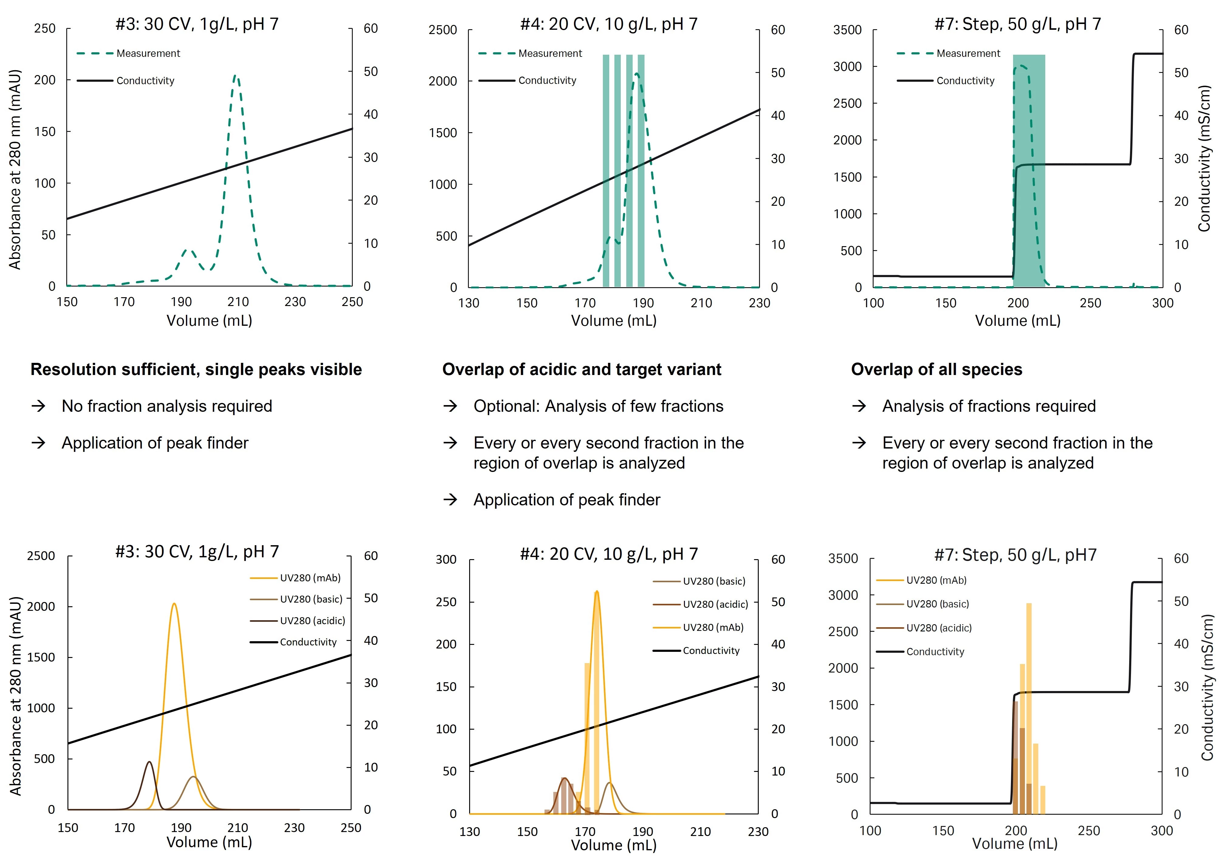
Fig 3. Peak finding tool
5. Data integrity check

The next step is to start building the virtual representation of the chromatographic process by importing data into GoSilico chromatography modeling software. A data integrity check should be performed before starting model calibration. The characteristics of the experimental data such as dead volumes and mixing effects in the system need to be accounted for to model the conductivity trace accurately.
Case study
The first step in representing the process digitally is to set up the properties of the biomolecules, system, and column in the software. Next, methods and experimental results are exported from UNICORN™ software and imported into GoSilico chromatography modeling software. Suitable data formats are .zip, .res, and .xlsx or .csv. Typically, UV sensor data, conductivity, and pH traces are imported.
A conductivity check is performed by comparing the imported conductivity traces to the simulated conductivity traces to ensure that system dead volumes and mixing effects are captured correctly. Especially for step elutions, the point of conductivity increase needs to be captured correctly. The simulated and measured pH values are compared in a similar manner — this is especially relevant for pH-sensitive processes or pH-induced elution.
Find more information on the conductivity check here.
6. Select a model

A mechanistic model for liquid chromatography accounts for the fluid-dynamic phenomena of system and column as well as the thermodynamic phenomena describing the interaction of biomolecules and ligand. Model selection follows a bottom-up approach. The selected column, pore, and isotherm models should be as simple as possible and only as complex as necessary. It is important to describe the present effects while avoiding overparameterization by choosing complex models with physically unreasonable parameters for the project at hand.
Find a general guide to model selection here.
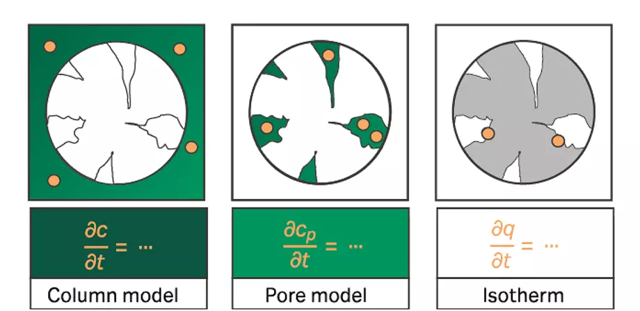
Fig 4. Fluid-dynamic and thermodynamic models
Case study
First, a model to describe the fluid-dynamic effects is selected. The combination of a transport dispersive column model and a lumped rate pore model accounts for the effects of convection, axial dispersion, and mass transfer. The mass transfer of the component from interstitial to pore volume is accounted for by a lumped film diffusion coefficient.
To describe the thermodynamic interactions of ion-exchange chromatography, we recommend using the colloidal particle adsorption (CPA) model . The following requirements need to be met for the separation problem at hand:
High load density should be modeled accurately:
The CPA model describes the elution behavior in both the linear and nonlinear range of protein loading and has shown superior performance and good accuracy for high load densities. High load densities can result in unusual, shoulder-like, trapezoidal peak shapes, which the CPA model can describe accurately as seen in Briskot et al. (1).
Dependency of pH on the process needs to be described:
The CPA model describes the pH influence on binding by means of a second order polynomial, which accounts for the influence on surface charge. Briskot et al. (1) has shown the CPA model to be an accurate choice for a pH dependent process over wide and small pH ranges.
7. Calibrate your model

Model calibration, or parameter estimation, is the process of measuring or mathematically estimating parameters of generally applicable model equations to represent the actual physical system. The input data used for model calibration are the wet-lab experiments and the respective offline analytical data. The aim of calibration is to identify model parameter values such that the simulated measurements match the experimental measurements. Certain attributes of chromatograms contain information about certain parameters. Ideally, this fact should be used for parameter determination to avoid parameter correlations and unreasonable parameter estimates without physical meaning.
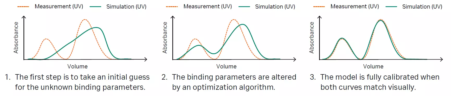
Fig 5. Model calibration
For example, ion-exchange chromatography linear gradient elutions (LGE) at low column loading can be used to determine the biomolecule charge and the equilibrium constant using the Yamamoto approach. To do so, at least two, ideally three LGE experiments featuring different gradient lengths are needed to determine the charge and equilibrium constant from the gradient slopes and the salt concentration at peak elution. The Yamamoto approach is readily available in GoSilico chromatography modeling software .
After the charge and equilibrium parameters are identified, other parameters such as the binding kinetics and pore diffusion characteristics can be determined from a step elution experiment, for example. The biomolecule-ligand interaction at high load density, displacement, or repulsion between the biomolecules can be determined from an additional high loaded LGE. This step-by-step approach will mitigate the risk of unreasonable correlations and unrealistic physical parameter estimates.
Find a general guide to model calibration here.
Case study
The CPA model distinguishes between resin parameters and biomolecule parameters. In total, 35 yet unknown parameters need to be identified:
3 resin parameters
8 biomolecule parameters × 4 biomolecule species* = 32 parameters
*target mAb, basic variant, two acidic variants
While this sounds like a large number, the optimization problem of mathematically estimating these parameters can be significantly reduced by conducting the following steps.
Step 2: deriving parameters from correlations, literature, or the RofA of the f(x) column
Due to the physical meaning of the CPA model parameters, measured values, correlations, literature values, or the results of analysis (RofA) sheet provided with all f(x) columns can be used to derive values for the parameters.
Table 4. Isotherm parameters
| Parameter name | Unit | Derivation |
| Ligand density | mol/m² | Resin parameter, provided with f(x) column |
| pKa Ligand | pH | Resin parameter, literature value |
| Colloid radius | m | Biomolecule parameter, derived from measurements or correlation of molecular weight and biomolecule radius* |
* for antibodies see Lavoisier and Schlaeppi (2)
This step reduced the optimization problem to:
1 resin parameter
7 biomolecule parameters × 4 biomolecule species = 28 parameters
Step 3: Yamamoto’s method
Yamamoto’s method uses linear gradient elution experiments at three different gradient slopes (run #1 to #3 and #8 to #11) as input to correlate gradient slope and salt concentration at peak retention. Based on this correlation, charge and equilibrium parameters can be derived.
Table 5. Isotherm parameters
| Parameter name | Unit | Parameter description | Derivation |
| Charge | - | Surface charge of biomolecule | Yamamoto’s method |
| Equilibrium | - | Thickness of interaction boundary layer | Yamamoto’s method |
| To include pH dependency: | |||
| Charge 1 | - | Accounts for pH-dependent biomolecule charge, slope of titration curve | Yamamoto’s method |
| Charge 2 | - | Accounts for pH-dependent biomolecule charge, curvature of titration curve | Yamamoto’s method |
While Yamamoto's method provided reliable parameter values in this case study, it is possible that these parameters need further refinement in form of mathematical estimation with optimization algorithms for other cases.
This step reduced the optimization problem further to:
1 resin parameter
3 biomolecule parameters × 4 biomolecule species = 12 parameters
Step 4: mathematical estimation
To derive the remaining parameters, the experiments using step elutions and higher load conditions (run #4 to #5) are used as additional input for mathematical estimation. Moreover, the initial guess for the specific adsorber surface is refined.
Table 6. Isotherm parameters
| Parameter name | Unit | Description | Derivation |
| Kinetic | 1/s | Biomolecule parameter, accounting for rate of adsorption/desorption | Estimation parameter |
| Lateral charge | - | Biomolecule parameter, accounting for interaction between biomolecules | Estimation parameter |
| Film diffusion | µm/s | External mass transfer between interstitial volume and particle pores | Initial guess derived from correlations (e.g., Wilson-Geankoplis) refined by estimation |
| Specific adsorber surface | m²/m³ | Resin parameter, adsorber surface accessible by biomolecules | Initial guess provided with f(x) column, refined by estimation |
Typically, the mathematical estimation starts with an algorithm screening a large parameter space, for example, with a heuristic algorithm such as adaptive simulated annealing. It is advisable to refine all model parameters using a deterministic algorithm (e.g., Levenberg-Marquardt). The number of parameters defines the dimensionality of the search space. Thus, to further break down the complexity for the mathematical solver, start with the estimation of model parameters for only the target species (species with highest concentration) first and then calibrate the impurities.
The model is calibrated when experimental and simulated traces match, as seen in the chromatograms in Figure 6.
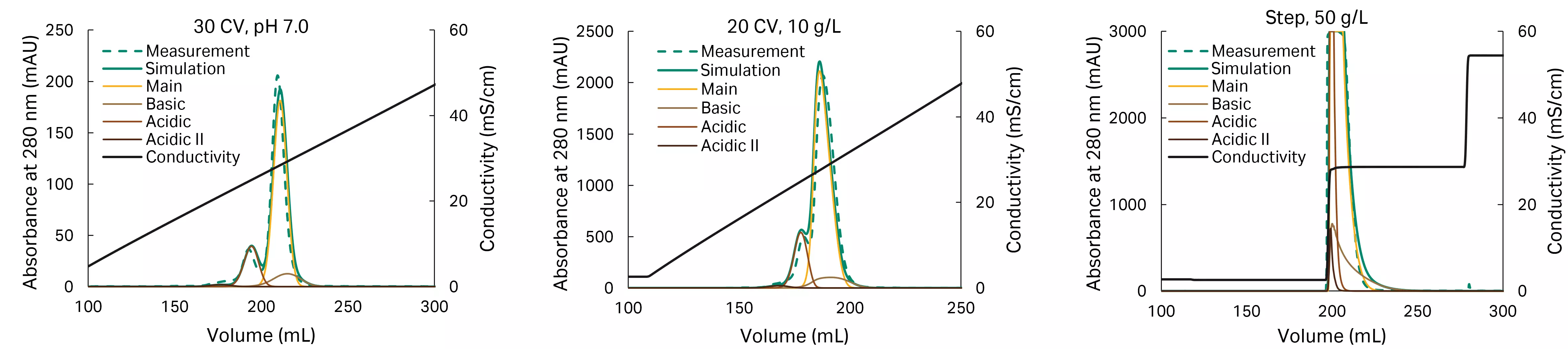
Fig 6. Calibrated model, from left to right: run #2, run #4, and run #7
8. Analyze parameter uncertainty

After model calibration, the model quality needs to be investigated. The first indicator for model quality is the visual fit. A high-quality model describes all calibration runs accurately.
Once a good visual fit is obtained, the model quality can be evaluated more intensely. To investigate the parameter sensitivity, the 95% confidence level needs to be determined. Those can be calculated directly in GoSilico chromatography modeling software. Well-determined parameters have narrow confidence intervals. Broad confidence intervals indicate that the respective parameters could not be determined accurately from the calibration data.
To investigate the influence of the parameter sensitivity on the model prediction, a parameter space sampling for the calibration experiments can be done within the calculated confidence intervals. This sampling will help determine if specific parameter sensitivities are sufficient. Based on the outcome of the parameter uncertainty analysis, additional calibration experiments can be performed to improve the model quality.
Case study
GoSilico chromatography modeling software supports the model quality assessment with different indicators and tools. In addition to assessing model quality, experimental model validation will follow in the subsequent step.
Visual fit
The visual match of experimental and simulated traces can be investigated qualitatively by visually comparing simulation and experiment in the software. Additionally, a quantitative evaluation of the visual fit using the R² value is possible.
Confidence levels
Typically, the confidence intervals of all relevant estimated parameters are calculated and displayed in form of violin plots, as depicted in Figure 7. The narrower the depicted violin plot, the higher the confidence. Broader confidence intervals, visualized as broader plots, indicate more uncertainty in the determined binding parameters. The interpretation of the calculated absolute values allows you to assess the risk associated with each uncertain parameter. As example, the basic variant, which is a noncritical impurity, has a higher uncertainty in the binding parameters. So the risk of having a potentially less accurate prediction for this noncritical impurity is acceptable. Contrarily, the uncertainty for the parameters describing binding of the target molecule should be relatively low to ensure good predictions for the component of interest.
The next step is to run a sampling based on the calculated covariances. This means that for each variable for which the model confidence was assessed, a normally distributed sampling around the mean value of the respective variable is performed. The width of the distribution is based on the calculated confidence intervals. By overlaying the resulting chromatograms, the impact of model uncertainty can be visualized. The plot in Figure 7 shows an overlay of 100 runs, indicating robust model parameters (depicted as it would be seen in GoSilico software).
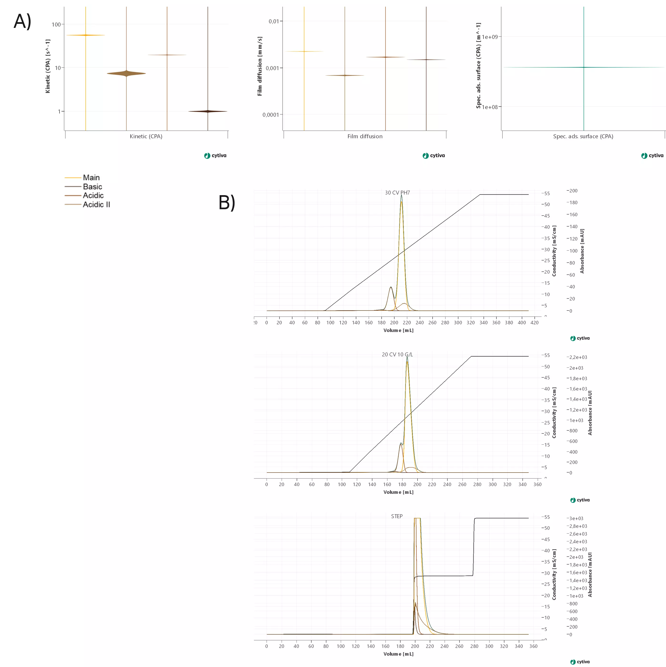
Fig 7. Model quality check. A) violin plots visualizing the confidence intervals of selected model parameters. B) Overlay of 100 sampling runs for three calibration experiments.
9. Validate your model

Once the model is calibrated, the model must be validated experimentally. The model validation can be done with one or multiple experiments. A common approach is to perform model validation with in silico optimized process conditions. Another possibility is to choose process conditions at the edges of failure of the model. It is also possible to include experiments at different scales for model validation if all used systems and columns were characterized.
The validation is typically done with respect to peak shapes and positions as well as critical quality attributes. The validation runs can be imported to GoSilico chromatography modeling software to compare experimental data and model prediction.
Case study
The model is validated with a two-step process at center point conditions (pH 7) and a 21.5% B concentration for the first elution step. The experimental method determined during in silico process optimization was executed as wet-lab experiment. Peak shape as well as the results of the analytics performed on the collected pool were evaluated. The predicted and experimental UV trace show a good match. Purity is predicted very well (model prediction: 96%, experimental validation: 97%) and yield shows a good match (model prediction: 87%, experimental validation: 83%) with an acceptable offset between model prediction and experimental validation.
In any case, the variation of the analytical method(s) used to confirm the model predictions should be considered when assessing whether the prediction was successful. For example, if particular assays come with error bars of 15%–20%, you should decide on an acceptable offset.
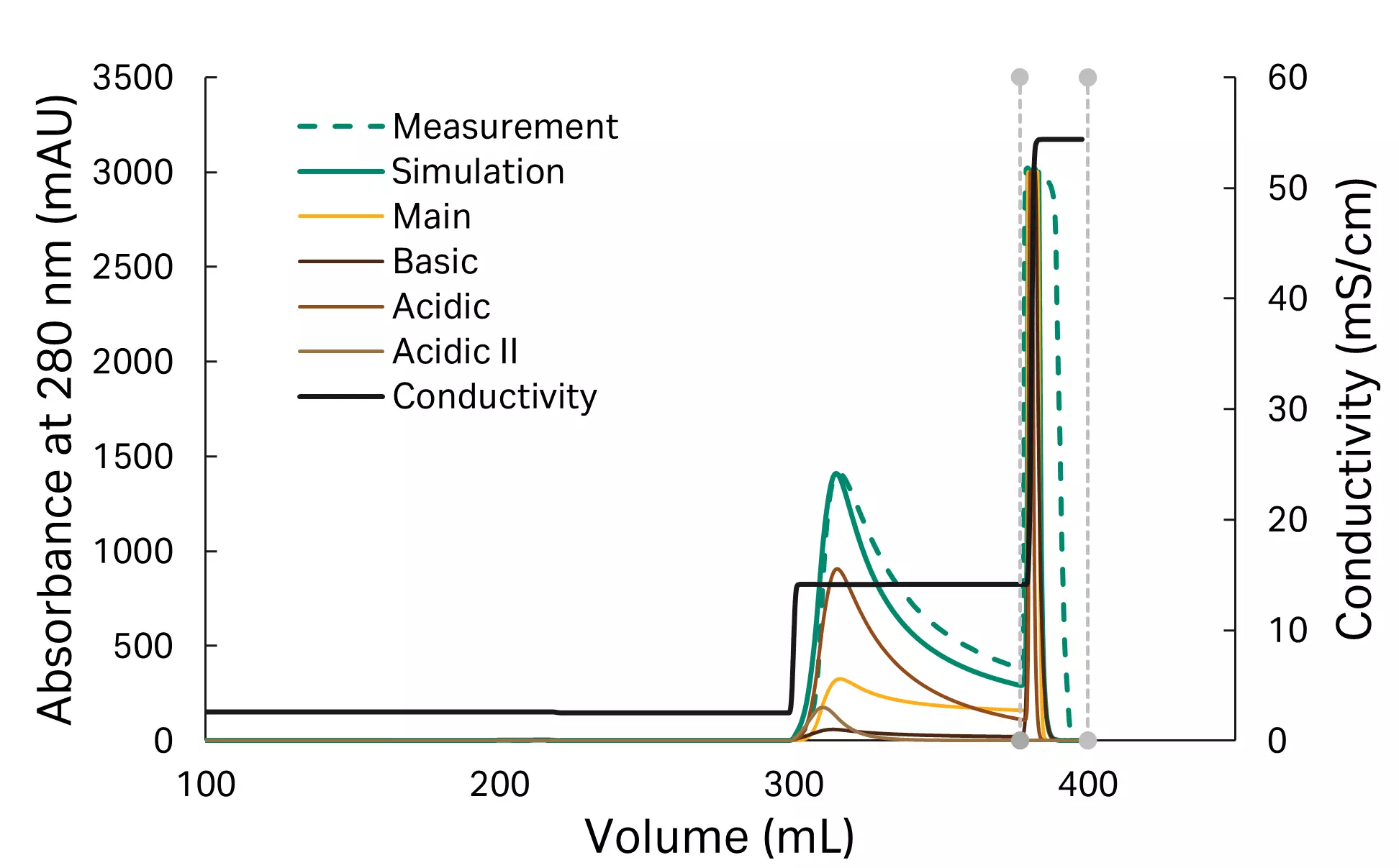
Fig 8. Model validation
10. Apply and further develop your mechanistic model

Once successfully calibrated and validated, the model can be used along the entire development life cycle of the product and process. Validated mechanistic models can extrapolate to process conditions outside the calibration space.
To guarantee a suitable ratio between effort and benefit, keep the desired model application in mind during the whole modeling workflow as different model purposes result in different implications regarding model quality and capability.
Read more about model applications examples here.
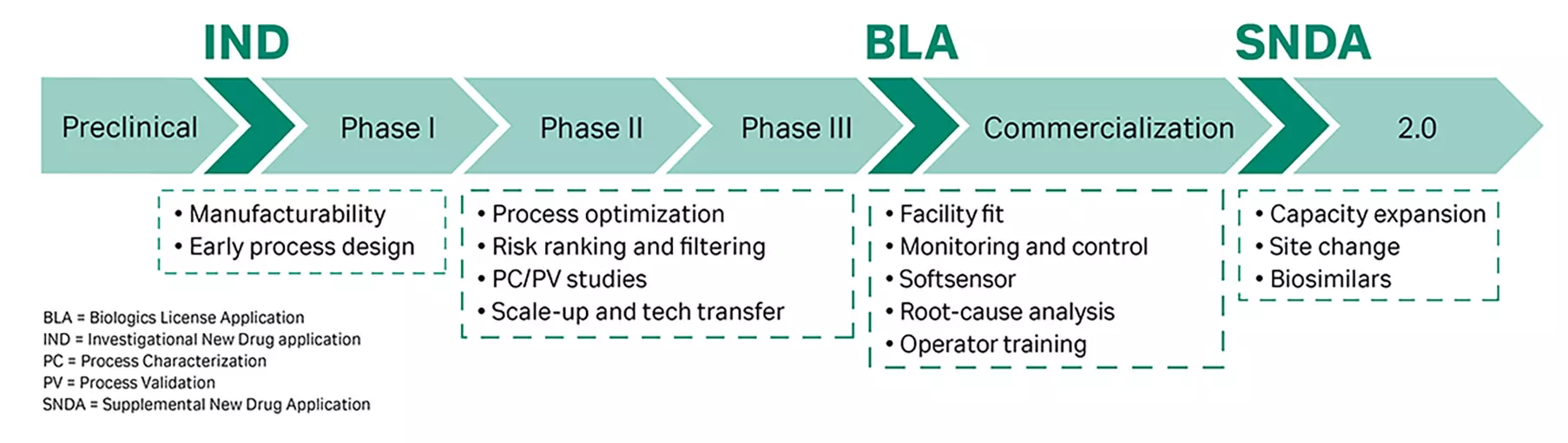
Fig 9. Model applications along the lifecycle of a biomolecule
Case study
An in silico process optimization was performed to achieve high yield and purity of the target species while keeping the elution volume small and load density high. Therefore, variable process parameters such as the process pH value and the salt concentration of the first step, load density, and method phase length were selected as variables. The best run was validated experimentally.
For process optimization, GoSilico chromatography modeling software aims to maximize an objective function by altering selected variables within defined boundaries.
Objective function
GoSilico chromatography modeling software allows you to set up the objective function using various objectives (yield, purity, quantity of biomolecule, self-defined objectives, etc.) and connect those via mathematical operators.
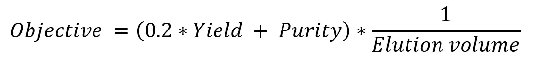
This way, objectives can be weighted. For example, for the polishing step at hand, purity is the most relevant objective while maximizing yield and minimizing elution volume.
Variables and boundaries
| Variable | Boundaries | Best run |
| % B concentration of the first elution step | 10–60 % B | 25.4%, equal to 152 mM NaCl |
| Elution volume of both steps | 3–10 CV | First step: 6.5 CV Second step: 5.0 CV |
| Load density | 50–90 g/L | 80 g/L |
Analytical evaluation of the best run’s fractions shows very good agreement of prediction and experimental validation. Thus, the final process met all acceptance criteria, achieving a purity of 97% while maintaining a yield of 86%. The elution volume of the first step could be further reduced to 6.5 CV, compared to the validation run with 10 CV elution volume.
Analytical results (HPLC-IEX):
| Model prediction [%] | Experimental validation [%] | |
| Yield* | 83 | 86 |
| Purity† | 97 | 97 |
| Main, first step | 37 | 39 |
| Acidic I + II, first step | 58 | 60 |
| Basic‡, first step | 5 | 1 |
| Main, second step | 87 | 88 |
| Acidic I + II, second step | 3 | 3 |
| Basic‡, second step | 10 | 8 |
* Yield is calculated as follows: Y = quantity of main and basic in pool/quantity of main and basic in load
† Purity is calculated as follows: P = quantity of main + basic in pool / quantity of total biomolecule in pool
‡ Basic variant is defined as noncritical impurity.
Summary
This clearly defined, straightforward workflow facilitates the calibration and application of mechanistic models significantly by increasing the speed of model calibration, reducing the model uncertainty, and mitigating the risk of parameter overfitting at the same time. Following this approach allows mechanistic modeling to unfold its full potential as in silico process development tool.
References
- Briskot T, Hahn T, Huuk T, et al. Analysis of complex protein elution behavior in preparative ion exchange processes using a colloidal particle adsorption model. J Chromatogr A. 2021;1654:462439. doi:10.1016/j.chroma.2021.462439
- Lavoisier A, Schlaeppi J-M. Early developability screen of therapeutic antibody candidates using Taylor dispersion analysis and UV area imaging detection. MAbs. 2015;7(1):77-83. doi:10.4161/19420862.2014.985544